ARCHIVE · CORRECTED 28 SEPTEMBER 2026 — This is the first investigation, kept as it was. Its null results stand, but Phase 2 reads four of its measurements differently: R9’s coherence curve is an identity of how looks are cut (1 − Δ/W), not a property of the ground; R4’s 77 µm/s “floor” is the scatter of a reading that recovers about 1% of real ground motion; R7’s committed run never recovered its injected motion; and R10 inherits R9’s identity. The platform travels 187.6 km over the aperture (168 km was one bank’s centre span). Two steps of the argument below are superseded: step 3’s “one pass gives two seconds” came from R9’s identity (a pass lasts 24.5 s, and every current analysis uses all of it), and step 5’s array test added its wave after tracking (P2-09 puts it into the image, where the image’s virtual sensors do not hear it). The corrections · Underworld
SAR / DEPTH, TESTED

One radar image cannot map what is under the ground

Single-image SAR Doppler tomography, as published for the Great Pyramid in 2022 and announced for Khafre in 2025, reimplemented and run on two real ICEYE Spotlight Dwell Fine acquisitions of Giza and Sacsayhuamán. Sixteen measurements, eight simulations, three supporting benchmarks. Every figure is generated by code in the repository.

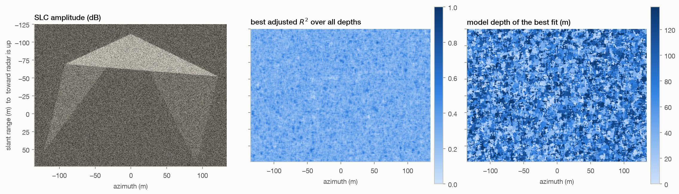
The idea is reasonable, and it fails on the recording, not on the arithmetic. A radar image does measure motion at millions of points, a denser array than any seismic deployment, and turning such an array into an image of what lies below is standard seismology. The obstacle is time. That method needs minutes of continuous recording; one radar pass yields under two seconds, because a radar builds its image from a sweep of angles and waiting a second also means moving a degree, after which the ground no longer looks like itself. We ran the array test regardless, on 759 elements across 1.8 km: an injected wave was recovered every time, the real data was flat. Separately, at the known depths of hundreds of surveyed burial shafts nothing appears; a pyramid and open desert score the same in one acquisition; X-band reaches about half a metre into limestone; and the depth axis is periodic by construction with a freely chosen scale.
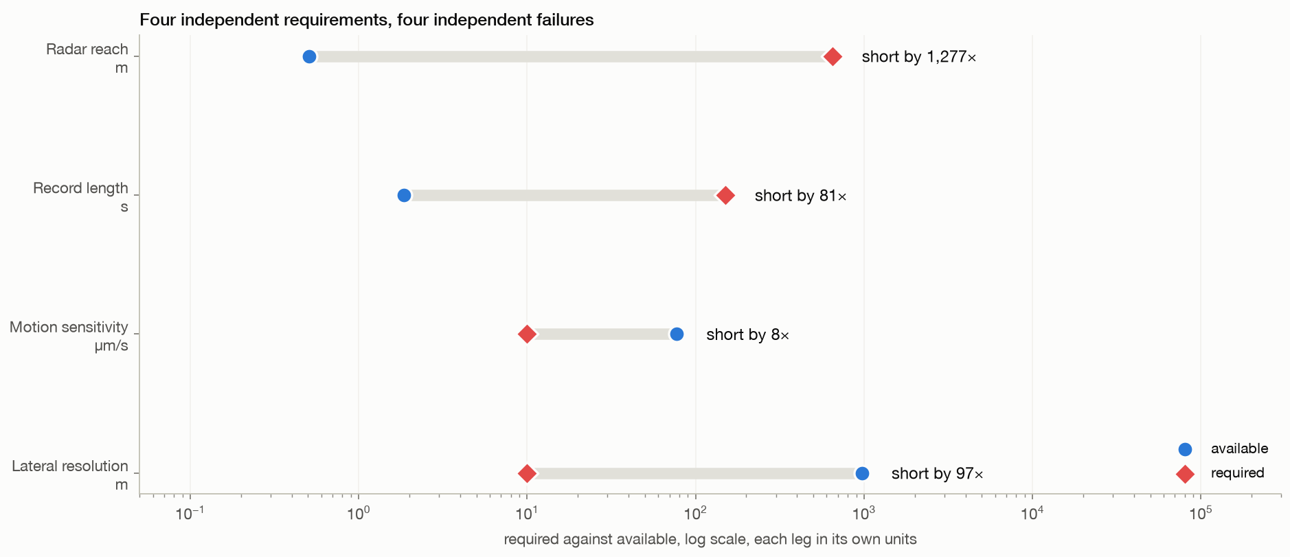
Radar reach1,277×

Short of what the claim needs. Required 648.0 m, available 0.51.

Record length81×

Short of what the claim needs. Required 150.0 s, available 1.86.

Motion sensitivity8×

Short of what the claim needs. Required 10.0 µm/s, available 77.39.

Lateral resolution97×

Short of what the claim needs. Required 10.0 m, available 972.00.

Known voids+0.031

Standardised difference between hundreds of surveyed burial shafts and bare plateau, at the shafts' own depths.

Array test0.004

Peak cross-correlation between array elements on real data. An injected wavefield gives 0.49.

Interactive · WebGL

The depth volumes, in three dimensions

Real output from the Giza acquisition. Compare a pyramid with empty plateau directly.

surface at the top · depth downward
drag to rotate · scroll to zoom

Patch

Rendering

chamber passage muon-detected void

lowhigh

This volume

What you are looking at. The grey plane on top is the real radar image of that patch, at 27 cm sampling. Everything below it is what the published method outputs as depth, rendered as a volume. The red plane marks where that output starts repeating exactly, because the steering basis has come back to itself. Switch between a monument and open ground, or between Giza and Sacsayhuamán: if the method were responding to buried structure, these would not look alike. On Khufu and Khafre the wireframes are the real chambers, passages and muon-detected voids, placed from excavation surveys and published muon imaging rather than from the radar; the volume simply repeats past them. On the cemetery patches a green band marks the depth range of hundreds of excavated burial shafts. Open the full viewer ↗

The argument

Six steps, each one measured

Including the strongest form of the idea, stated fairly before it is tested. Every step links to the experiment that establishes it.

01Radar does not go through rock

At this wavelength the signal dies about half a metre into dry limestone. Nothing underground is lit up. So anything the method knows about what is down there has to be read off how the surface moves.

02So far the idea is reasonable

A radar image gives a measurement at every pixel, millions of them, metres apart. That is a denser array than any seismic deployment on Earth. Shaking from distant oceans and cities passes through the ground everywhere, and seismologists routinely turn such an array into an image of the structure below. This is the strongest version of the claim, and it is worth taking seriously.

03Using it as a seismic array needs minutes, and one pass gives two seconds

Turning an array into a picture of what lies below means watching waves travel, and those waves have periods of several seconds, so the recording has to run for minutes. A radar pass builds its image from a sweep of angles, and time and angle are the same axis: to wait a second you must also move a degree, and after about a second the ground stops looking like itself. Measuring one displacement precisely is a different matter and needs no time at all.

04Sharper measurement does not help, because precision is not the limit

This scan resolves motion to 77 millionths of a metre per second, better than the published figure for a single pass. The trouble is that reaching a chamber needs a short, fast wave, and sampling a fast wave needs short slices of the pass, which widen every pixel by the same factor. The two demands pull apart. The smallest thing this acquisition could ever resolve this way is about 52 metres. Giza's chambers are metres.

05We ran the array test anyway, and nothing arrives

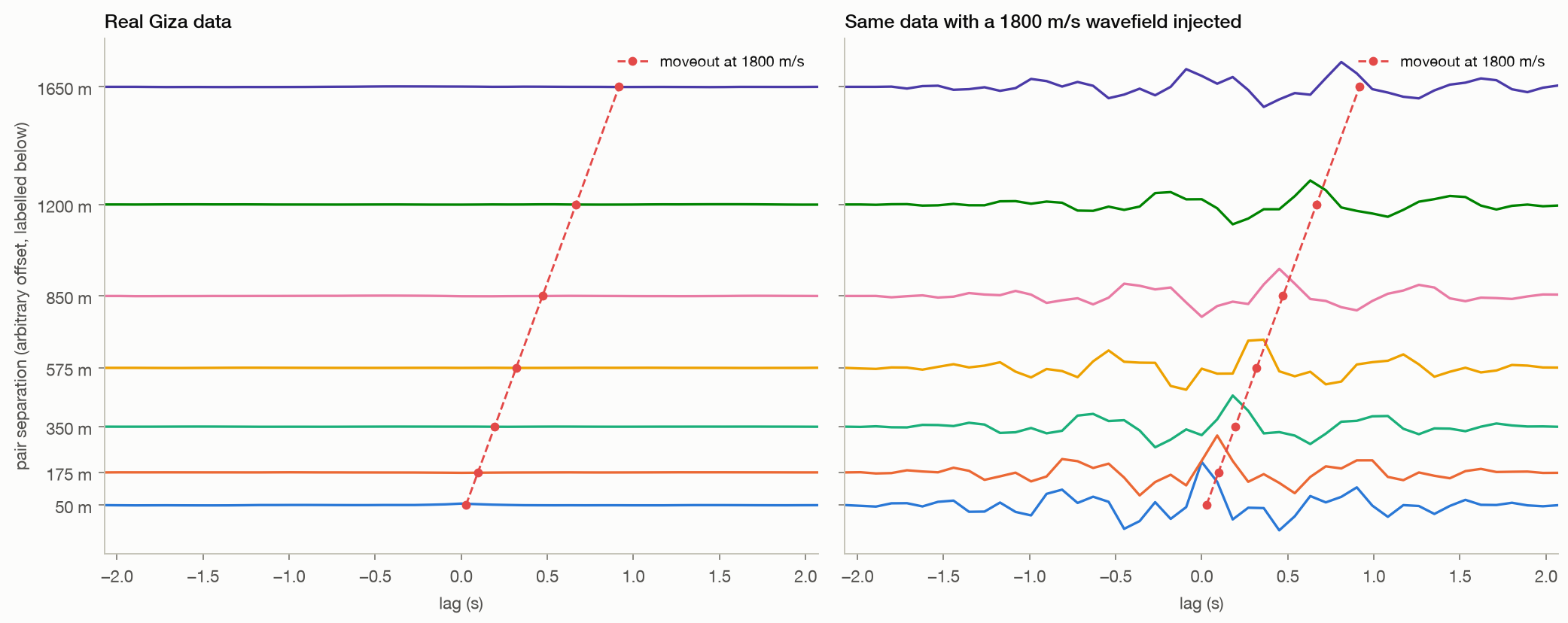
Seven hundred and fifty-nine elements over 1.8 km, cross-correlated in pairs and stacked by distance, exactly as a seismologist would. A wave shows up as a peak that arrives later the further apart the pair is. We injected one into the same data and the method found it every time. The real data is flat.

06Where voids are certainly known, nothing appears either

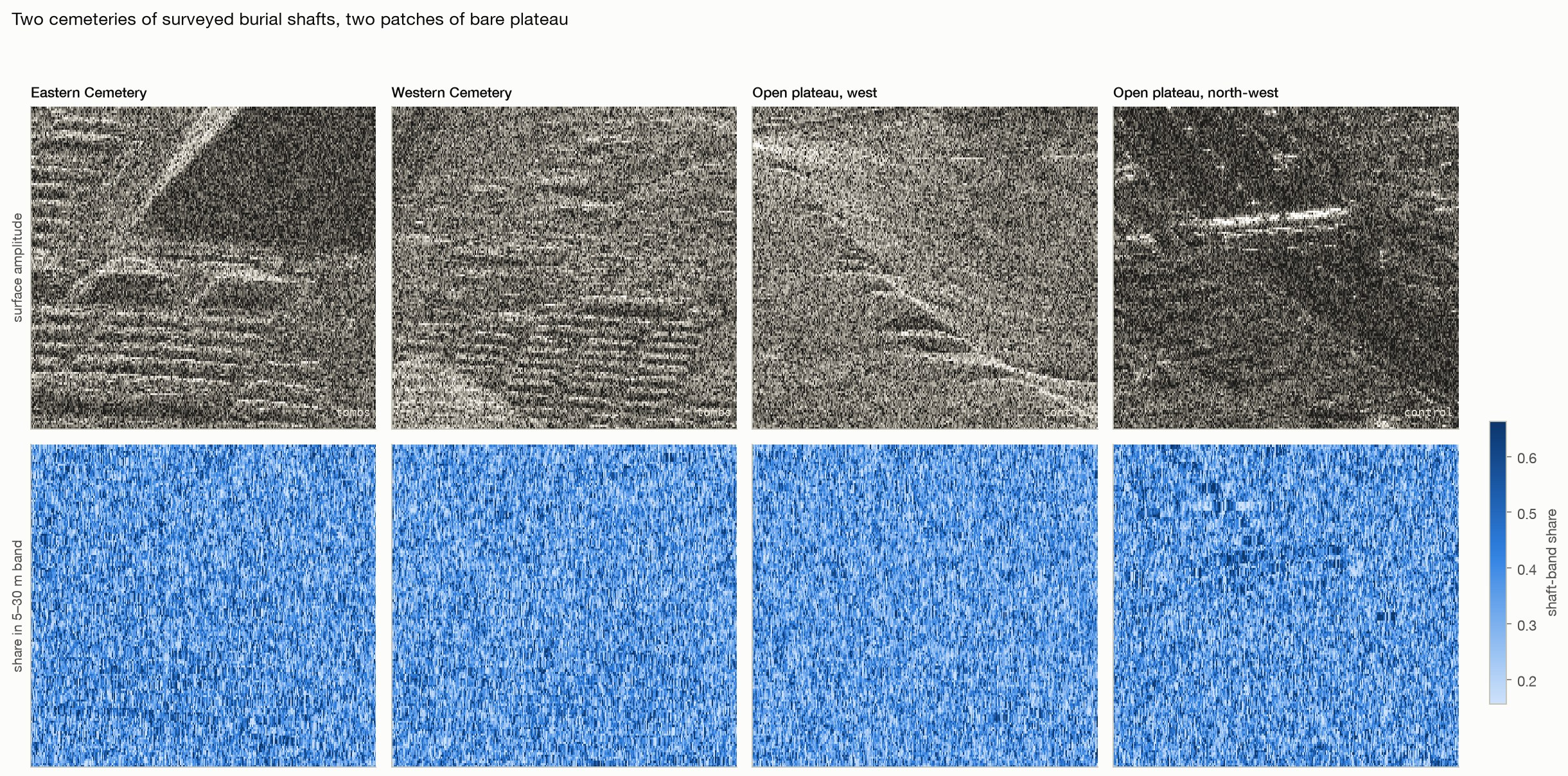
Giza's cemeteries hold hundreds of excavated burial shafts five to thirty metres deep, next to bare plateau with none. At the shafts' own depths, the two are indistinguishable.

07And the depth numbers are manufactured

The depth scale is set by a constant nobody measures, and the picture repeats every few metres. Two halves of the same pass put the same ground at different depths.

08The repeat is in the equation, not the data

The depth stage matches each pixel against a sine and a cosine of depth. Those two curves come back to the same pair of shapes at regular spacing, so a peak at one depth has an identical twin below it, and another below that. The method's own documents say so. The elliptical part people call the spring model runs earlier and only chooses which pixels get scored, so it cannot break the tie.

The data

What the radar recorded

Ten patches, two acquisitions, no processing. Every later result is a statement about these pixels.

Ten patches of two ICEYE dwell acquisitions
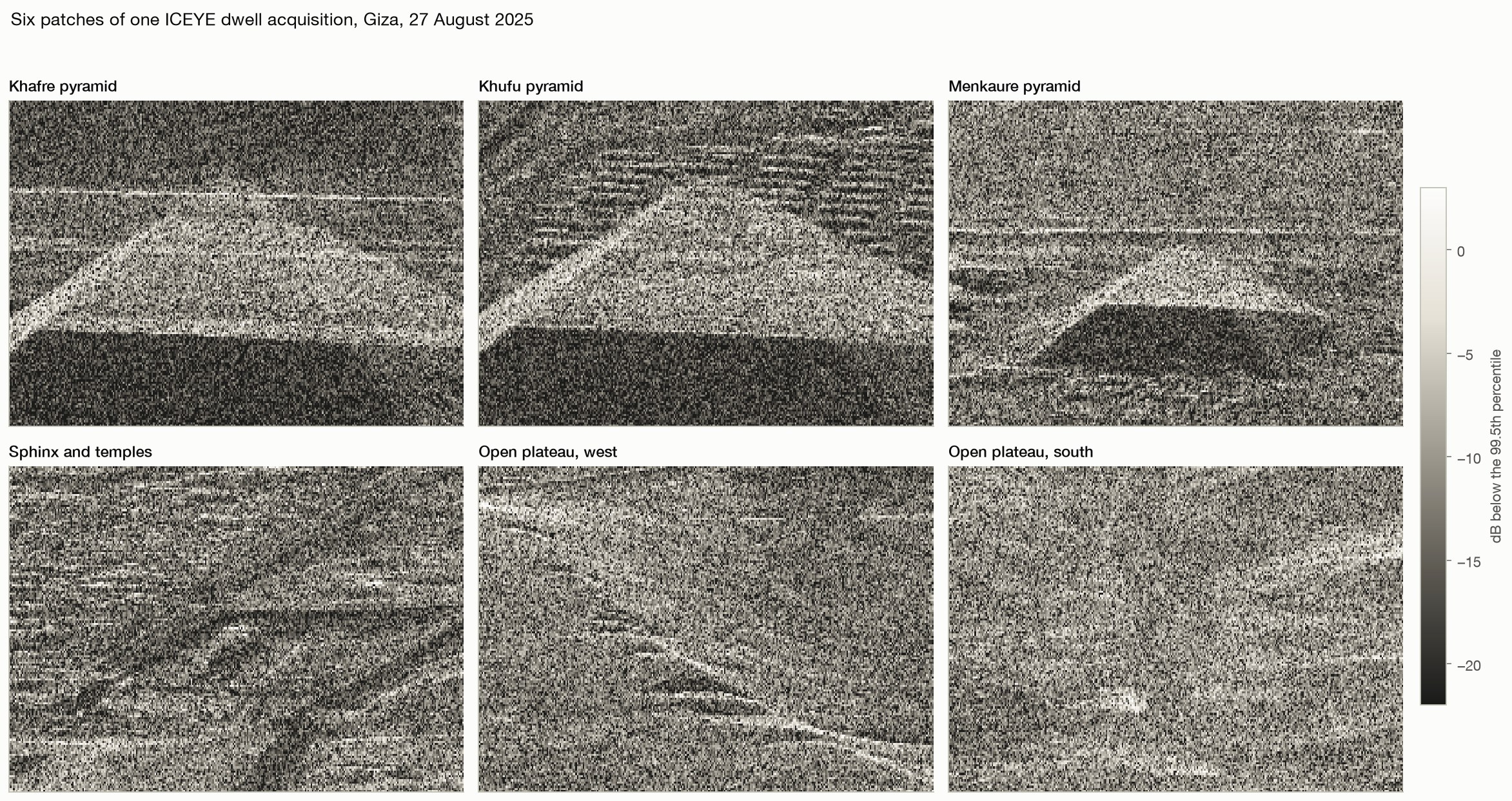
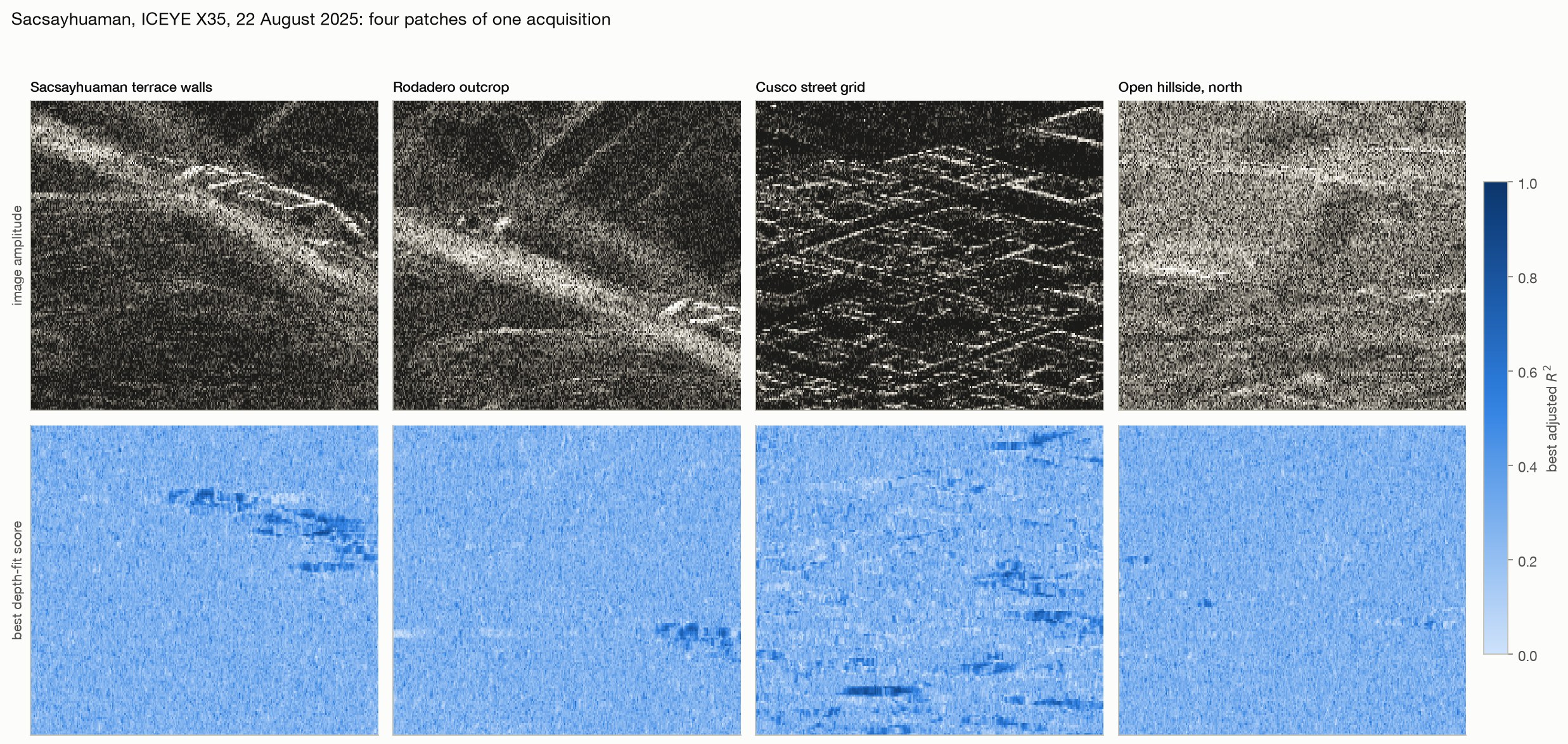
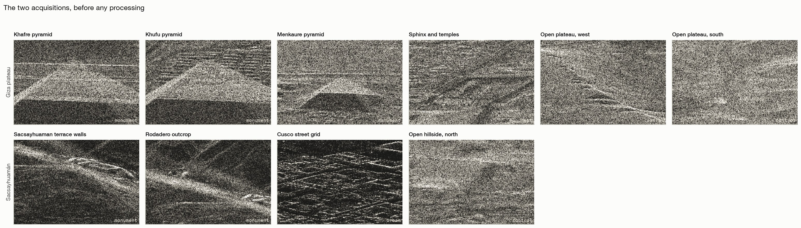
What the radar recorded. Amplitude of the native complex images on the analysis grid, geolocated by each product's own rational polynomial model with no fitted offset. Top: four Giza monuments and two stretches of open plateau, all inside one 25 second acquisition. Bottom: the zigzag terrace walls of Sacsayhuamán, the Rodadero outcrop, the street grid of Cusco and an open Andean hillside, in a second acquisition from a different satellite. The surface tells these apart at a glance. Everything that follows asks whether the depth output does.
Giza plateauICEYE-X33 · 2025-08-27 · 113,692 × 11,562 samples · 24.8 s · 20.8° incidence · 6 patches
SacsayhuamánICEYE-X35 · 2025-08-22 · 114,606 × 11,482 samples · 20.2 s · 20.5° incidence · 4 patches
Measurement · 16 tests

What the real acquisitions show

The budget first, then the positive control, then what the method distinguishes, then why, then whether our own code is to blame. Figures enlarge; method and limits are collapsed.

Every leg fails on its own. For the published claim to hold, four separate things must be true at once. The ra
14 · The budget

Four independent requirements, each missed by a wide margin

X-band penetrates 11 to 51 cm of dry limestone, so nothing below the surface is illuminated and every claim must rest on surface motion.

  • Resolving the microseism band needs a record of order 150 s; the coherent window allows 1.86 s.
  • Ambient ground motion is 0.1 to 10 µm/s; the measured floor is 77 µm/s.
  • Surface waves long enough to sample 648 m cannot resolve better than about 972 m laterally, against wells said to be 10 m across.
  • Each leg fails alone, and they are independent.
radar reach1,277×
record length81×
motion sensitivity8×
lateral resolution97×
Method, limits & data

Method. Penetration from the low-loss attenuation constant at 9.6 GHz for dry limestone. Record length and motion sensitivity measured in R9 and R4 on the real acquisition. Lateral resolution from the standard surface-wave depth-sensitivity and half-wavelength resolution relations.

Leaves open. Dielectric constants for dry carbonate rock span a range and the penetration figure moves with them, but not by the three orders of magnitude the claim would need. The resolution leg assumes surface-wave sensing; a body-wave method at the frequencies needed to resolve ten metres cannot reach the depth at all, so that route is worse rather than better. The record and sensitivity legs are measured on one sensor and one scene type.
Code ↗ · Results JSON ↓

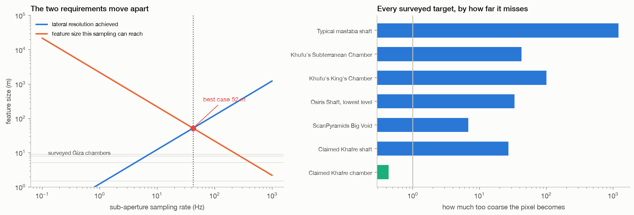
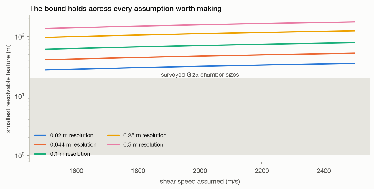
Sampling fast enough to hear a chamber makes the pixel too wide to find it. Left: the blue line is the lateral
16 · The resolution bound

Phase precision is not the limit, and improving it changes nothing

Because precision is not the binding constraint.

  • This dwell's own velocity floor is 77 micrometres per second, about 13 times better than the roughly 1000 micrometres per second reported for single-pass micro-motion on bridges, so this work agrees with that literature rather than disputing it.
  • The limit is a trade between two uses of one knob.
  • Reaching a feature of size s through the ground needs an elastic wave no longer than about twice its size, so at least Vs over 2s in frequency, and recording that frequency needs sub-apertures short enough to sample it; but azimuth resolution is inversely proportional to integration time, so every factor gained in sampling rate is paid for in lateral resolution.
  • Requiring both leaves s squared at least equal to azimuth resolution times aperture length times shear speed, putting the smallest resolvable feature here at 52 m, and never below 27 m across every assumption worth making.
  • That rules out every chamber actually surveyed at Giza.
smallest resolvable52 m
our motion floor77 µm/s
vs published13× better
Method, limits & data

Method. Aperture length, platform speed, slant range and wavelength were read from the ICEYE Giza product. Azimuth resolution was taken as the more favourable of the geometric value 0.050 m and the delivered pixel spacing 0.044 m. The bound is the square root of that resolution times the 24.8 s aperture times shear speed, evaluated at 2200 m/s and swept across 1500 to 2500 m/s and across azimuth resolutions from 0.02 to 0.5 m. The velocity floor is the measured value from R4; the comparison figure is the published single-pass bridge result.

Leaves open. This is an analytic bound computed from the acquisition's own geometry, not a measurement, and it is a necessary condition rather than a sufficient one: clearing it would not by itself make the method work, since the depth axis and the coherence limit are separate failures. It assumes a half-wavelength resolution criterion, which is the standard rule but can be beaten somewhat by a well-posed inversion with strong prior information. It assumes resolution scales inversely with integration time and that non-overlapping sub-apertures give one independent sample each, both of which are standard but idealised. It says nothing about methods that do not work this way, such as multi-pass interferometry over years, ground-based geophysics, or muon tomography.

Code ↗ · Results JSON ↓

No wave arrives. Velocity series recovered from a 1.8 km strip of the real Giza acquisition, cross-correlated
11 · The array

Used as a dense seismic array, the image contains no propagating wave to find

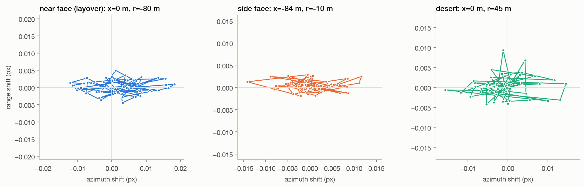
The first step already fails. Velocity series from 759 elements spread over 1.8 km were cross-correlated between pairs and stacked by separation.

  • Injecting a 1800 m/s band-limited wavefield of 400 µm/s into the same series is recovered on 5 of 5 informative separation bins, with a median peak correlation of 0.49.
  • The real data gives 0.004, lower by a factor of 120, and its peaks fall at unrelated lags.
  • Bins closer than about 350 m are excluded because neighbouring pixels share speckle and correlate at zero lag whatever the ground is doing.
  • The array processing works; there is no wavefield in the data for it to find, because the record is 2.1 s where the microseism band needs hundreds.
real0.004
injected wave0.49
Method, limits & data

Method. A 40,960 by 512 sample strip read from the native product, 24 common-reference sub-apertures of 8% bandwidth confined to the coherent window, azimuth shifts converted to line-of-sight velocity, pairs drawn at random within each separation bin and cross-correlated with each pair's zero-Doppler time offset removed before stacking.

Leaves open. One strip, one acquisition, one injected speed and band. The control is a single plane wavefield, which is easier to recover than a real diffuse ambient field, so this bounds the method from the favourable side. A longer record, from many tasked dwells stacked, would raise sensitivity at frequencies above about half a hertz; it cannot extend the record below that.
Code ↗ · Results JSON ↓

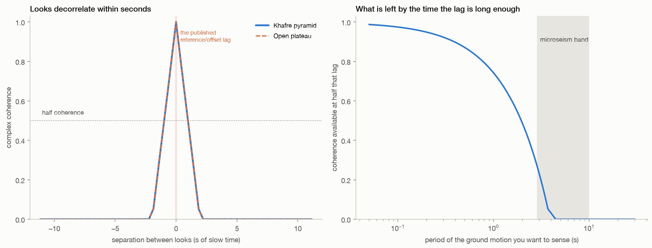
The constraint behind everything else. Left: complex coherence between sub-aperture looks of the real Giza acq
09 · The obstruction

In a dwell, time diversity and coherence are the same axis, and you cannot have both

No. Slow time and look angle are the same axis in a dwell product, so looks separated by seconds are separated by degrees, and natural ground decorrelates over a fraction of a degree.

  • Measured on the real acquisition, coherence with the band-centre look falls to half by 0.98 s of separation and to a tenth by 1.76 s, identically on the pyramid and on open desert.
  • Ground motion in the microseism band needs lags of about a second, by which point there is little coherence left to register.
  • The published protocols avoid this by using lags of tens of milliseconds, which keeps them coherent and makes them blind to the motion they invoke.
half coherence0.98 s
a tenth1.76 s
Method, limits & data

Method. 61 sub-apertures of 8 per cent bandwidth swept across the processed Doppler support of a real Khafre and a real desert crop; complex coherence computed against the band-centre look over the interior of each crop; separation converted to slow time through the product Doppler rate and to aspect angle through the carrier wavelength and platform speed.

Leaves open. Coherence is measured over one patch of one acquisition at 8 per cent sub-aperture width; a wider sub-aperture averages more and decorrelates differently. Strong stable point scatterers, such as corner reflectors or some built structures, hold coherence far longer than the natural desert measured here, so this curve is the distributed-target case, not a universal limit.

Code ↗ · Results JSON ↓

The mastaba rows are obvious; the shafts beneath them are not. Top: surface amplitude of the four patches, whe
13 · Positive control

Hundreds of surveyed burial shafts produce no signal at their known depths

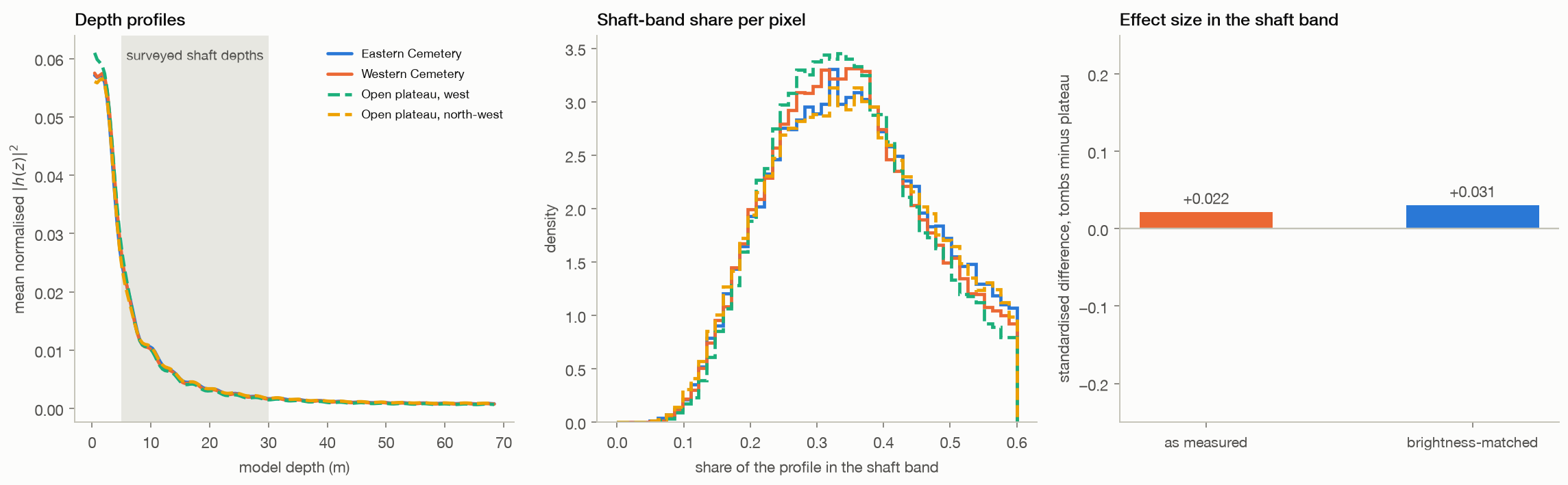
No. Across 95,760 pixels over the Eastern and Western Cemeteries and 95,760 pixels of bare plateau, the share of each pixel's depth profile falling in the surveyed shaft band of 5 to 30 m is 0.3736 over the tombs against 0.3706 over the plateau, a standardised difference of +0.022.

  • The cemeteries are far brighter at the surface, with median amplitude 67 against 77, so the comparison was repeated on brightness-matched pixels, where the difference is +0.031.
  • Any residual is accounted for by surface geometry: of the cemeteries' strongest surface periodicities that can reach this depth axis at all, 0 fall inside the band being tested, through the same spacing-to-depth relation the method uses.
  • This is the easiest target the site offers: shallow, numerous, excavated and surveyed, under flat ground.
tombs0.3736
plateau0.3706
matched effect+0.031
Method, limits & data

Method. Forty common-reference sub-apertures confined to the coherent window, chosen so the depth axis is unambiguous to about 67 m and the 5 to 30 m shaft band is representable, applied to two cemetery patches and two plateau patches of the same acquisition. The statistic is the fraction of each pixel's normalised depth profile lying in the 5 to 30 m band, compared directly and again after matching the two populations on surface amplitude in 24 bins.

Leaves open. The depth axis of this bank is unambiguous only to about 67 m, which covers the shaft band but not deeper claims. Shaft depths vary between tombs and many shafts are filled or collapsed, so the band is a range rather than a target depth. Placement is verified by recognising the mastaba rows in the image, not by surveyed control points, which is enough at this scale but would not be for a single chamber. A null here bounds sensitivity to shallow voids under these conditions; it does not prove no void anywhere could ever be detected.

Code ↗ · Results JSON ↓

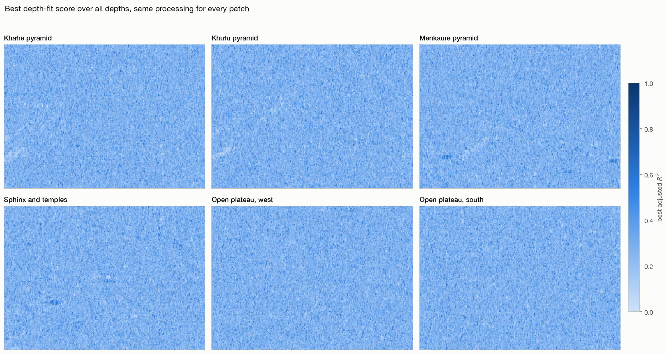
The six patches. Amplitude of the native complex image on the analysis grid, geolocated by the product's own r
01 · Within-image controls

Monuments and open desert give the same answer in the same acquisition

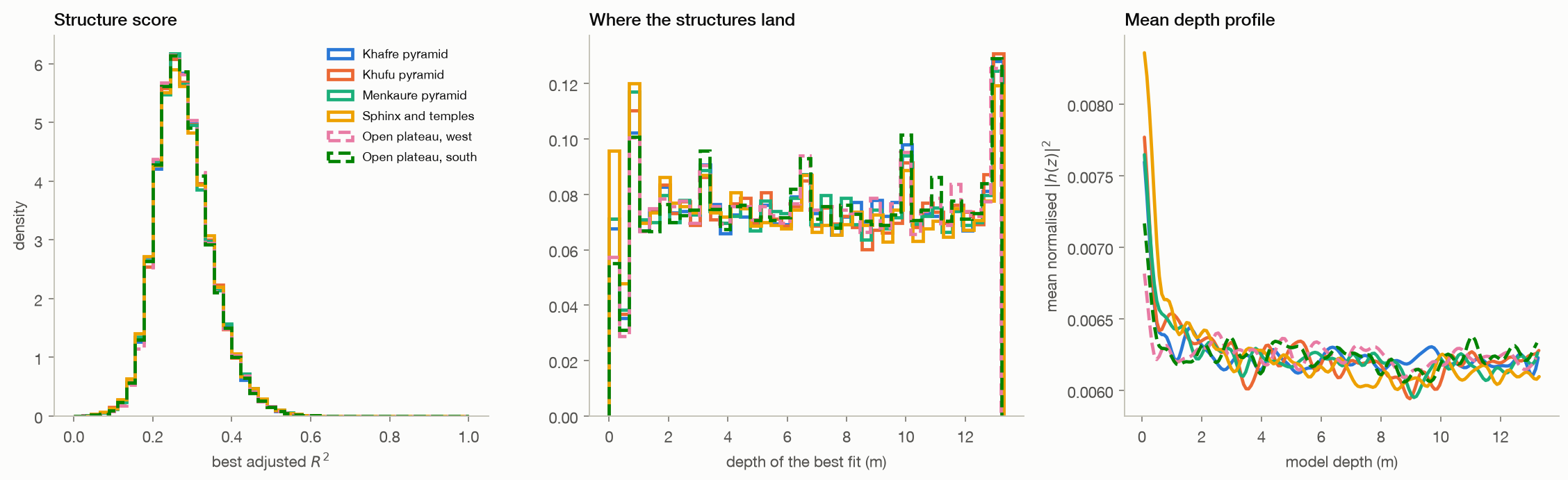
It does not. Across 191,520 pixels on four monuments and 95,760 pixels on two stretches of open plateau in the same acquisition, the mean structure score is 0.2798 on the monuments against 0.2803 on the desert, a standardised difference of -0.007, and it runs the wrong way.

  • The Kolmogorov-Smirnov distance between Khafre and the controls is 0.008.
  • Such a test returns a small p-value here only because the pixel count is large; the separation itself is under one percent of the score range.
  • The depth histograms and mean depth profiles have the same shape everywhere, and this bank's depth axis folds back at 13.7 m.
monuments0.2798
open desert0.2803
standardised gap-0.007
Method, limits & data

Method. ICEYE X33 Spotlight Dwell Fine, Giza, 27 August 2025, VV. Six patches of 4096 by 1536 native samples located by the product's rational polynomial model. Sub-aperture bank of 50 reference/offset pairs at half the processed bandwidth with an 88 Hz offset, 32 by 32 complex cross-correlation to a thousandth of a pixel, scene-median common mode removed, steering wavenumbers from the product's own state vectors, depth grid to the ambiguity limit.

Leaves open. Pixels inside a patch are not independent, so no p-value here should be read as a detection rate. This reproduces the published processing chain as described, on the same class of data, at patches we chose. It does not reproduce a specific published figure, because the bank parameters behind those figures were never disclosed. A difference in these statistics would not have proved a chamber either; it would have started a search for a surface cause.

Code ↗ · Results JSON ↓

A second site, the same outcome. Top: the native image amplitude, where the zigzag terrace walls, the Rodadero
06 · Second site

Another satellite, another continent, the same undifferentiated output

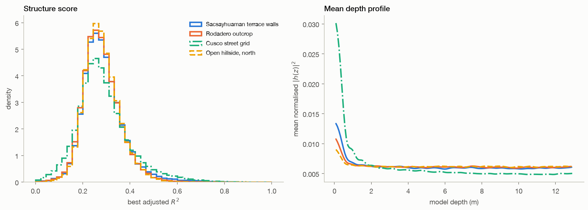
On the method. An ICEYE X35 dwell of Sacsayhuaman, a descending left-looking pass over the Andes at 3.6 km altitude, gives cut-stone terrace walls a mean structure score of 0.283, an open hillside 0.281 and the dense street grid of Cusco 0.286.

  • The Kolmogorov-Smirnov distance between walls and hillside is 0.014.
  • The depth axis for this acquisition repeats every 13.3 m.
cut stone0.283
hillside0.281
city0.286
Method, limits & data

Method. Identical pipeline, bank and grid to the Giza controls, applied to four patches of one ICEYE X35 Spotlight Dwell Fine acquisition of 22 August 2025, with steering wavenumbers from that product's own state vectors.

Leaves open. Steep Andean terrain makes single-height RPC placement much less precise than at flat Giza, so each patch was checked against the image rather than trusted from coordinates. No claim is made about what lies under Sacsayhuaman; this is a control on the processing.

Code ↗ · Results JSON ↓

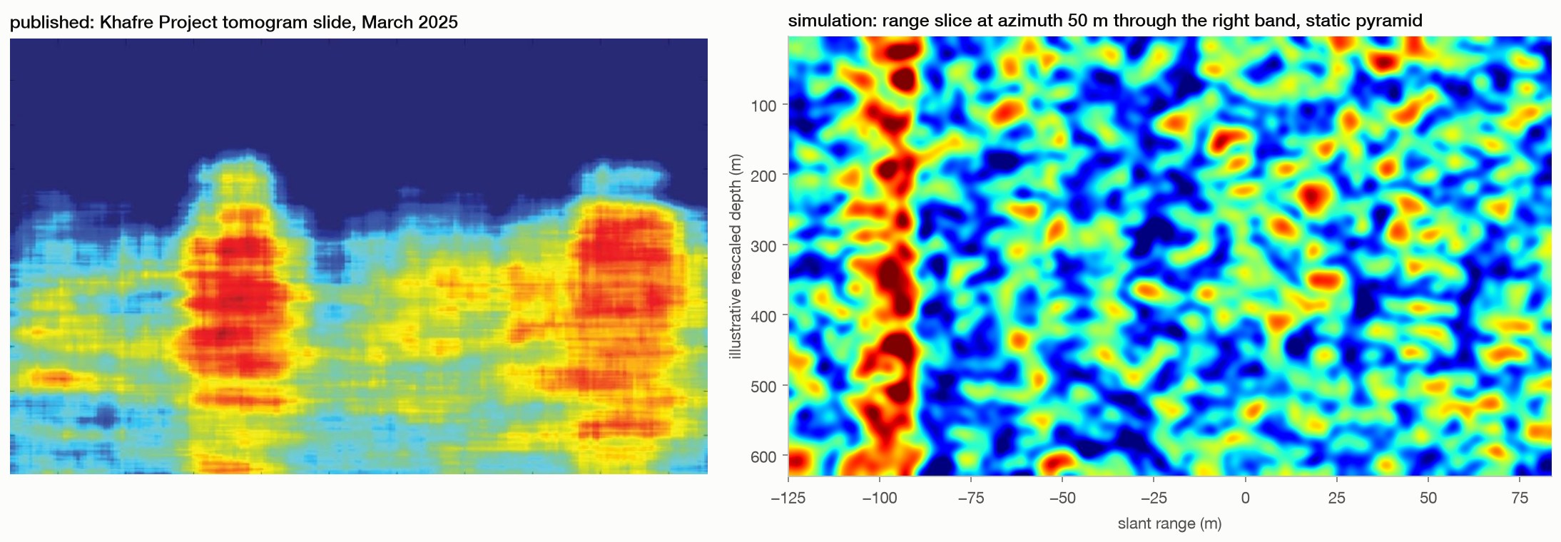
The view the slides showed, from the real acquisition. Top: the surface radar brightness along each strip, so
08 · The picture

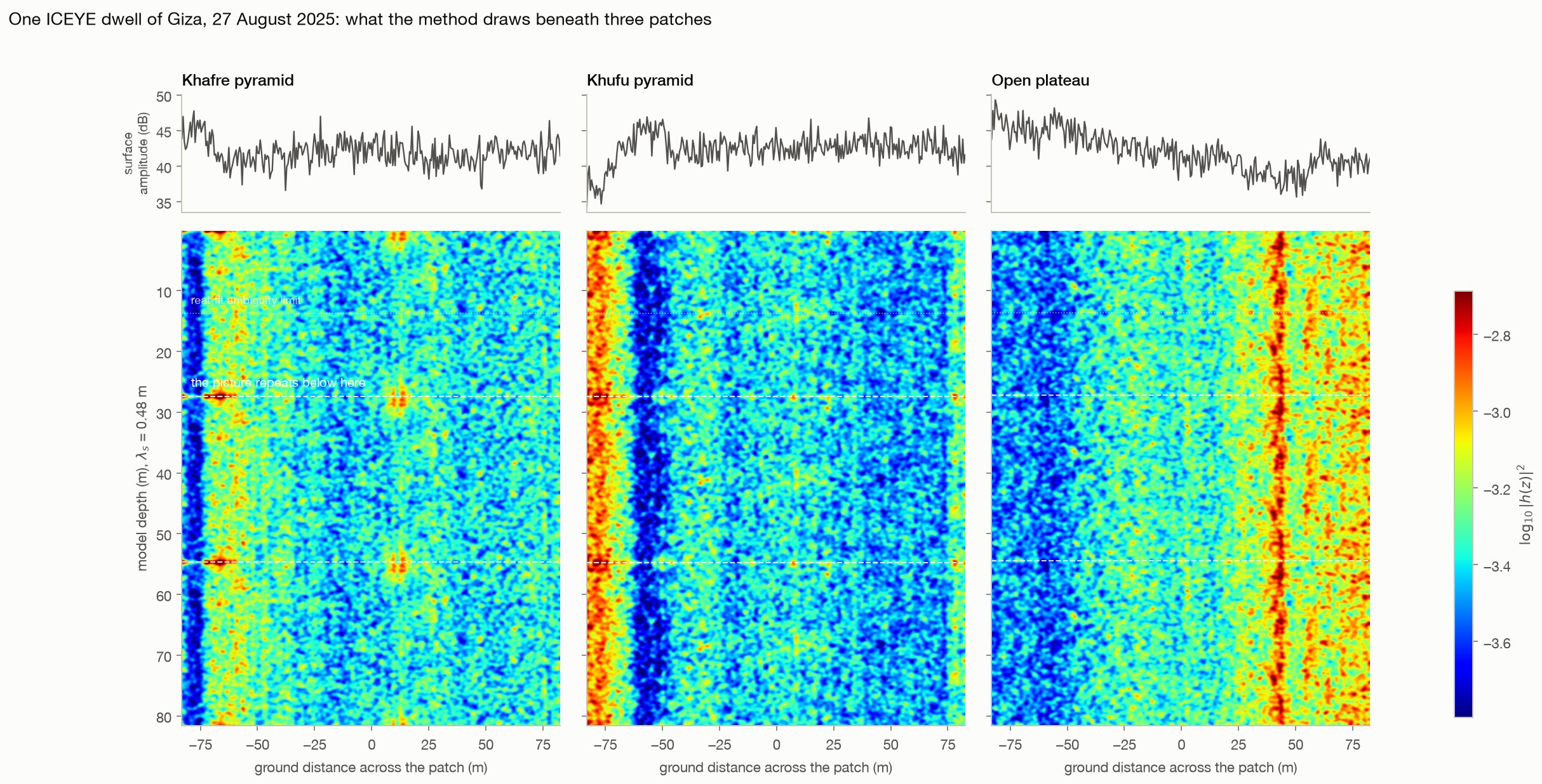
Rendered like the published slides, the real data shows the same thing everywhere

It looks like the published slides, under the pyramids and under empty plateau alike.

  • Vertical banded columns of the kind read as wells appear in all three patches of the same acquisition.
  • The steering wavenumbers are uniformly spaced to within a hundred-thousandth, so the section is exactly periodic: at Khafre it repeats every 27.4 m with a correlation of 1.000, meaning every structure drawn below that depth is a copy of one above it.
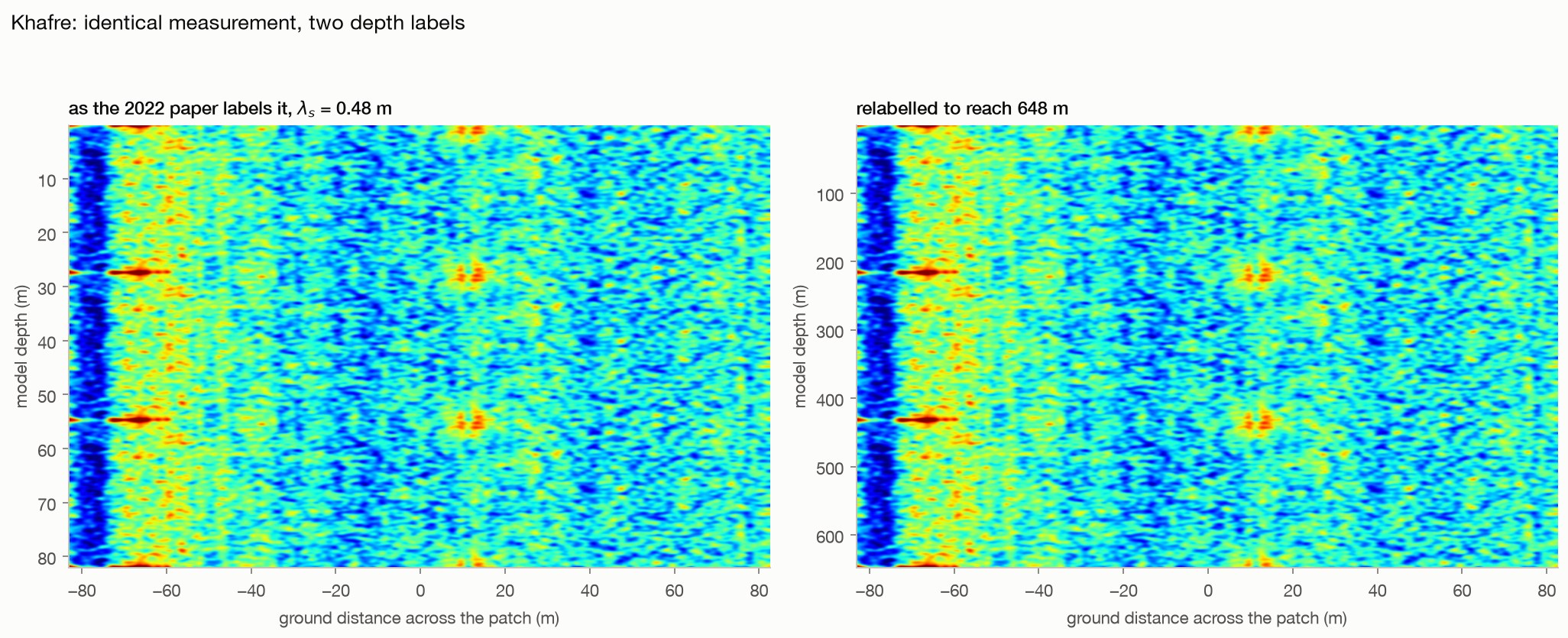
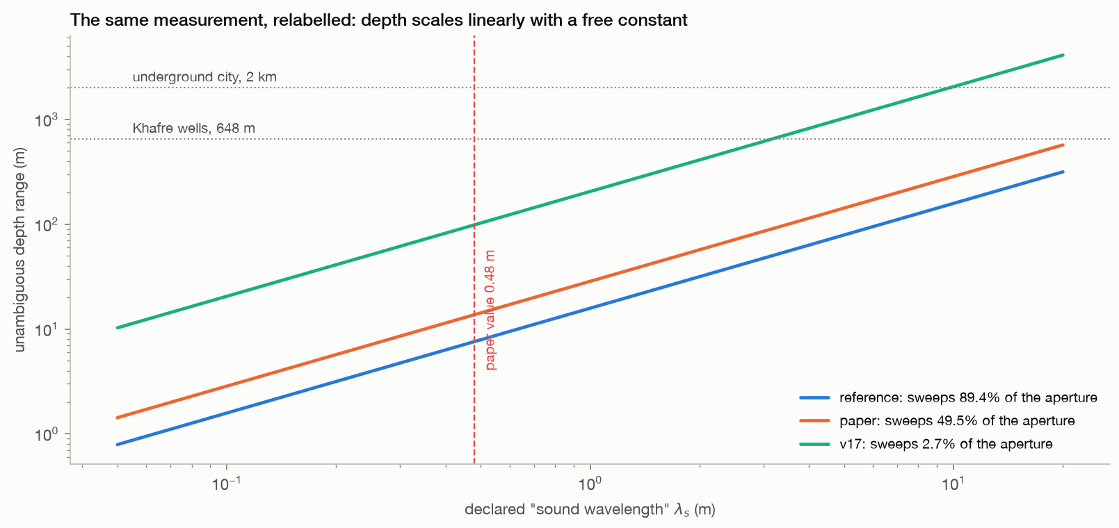
  • Relabelling the axis by declaring a sound wavelength of 3.8 m instead of 0.48 m puts the bottom of the same unchanged array at 648 m.
repeats every27.4 m
correlation1.0000
Method, limits & data

Method. Cached trajectories from the within-image control runs, refocused on a depth grid extended to three ambiguity periods, averaged over a band of range columns centred on the brightest part of each patch, smoothed and drawn in jet on one shared logarithmic scale.

Leaves open. These are our bank parameters, not the undisclosed ones behind the published images, so this is a like-for-like rendering of the method rather than a reproduction of a specific figure. The strips are 12 range columns wide and span about 165 m of ground, which is less than the full base of Khafre. Smoothing and colour scaling follow the published presentation, which flatters any such image.

Code ↗ · Results JSON ↓

The depth ceiling is bought by discarding aperture. Using real ICEYE state vectors at Khafre, the unambiguous
02 · Depth axis

The reachable depth is set by the sub-aperture bank, not by the ground

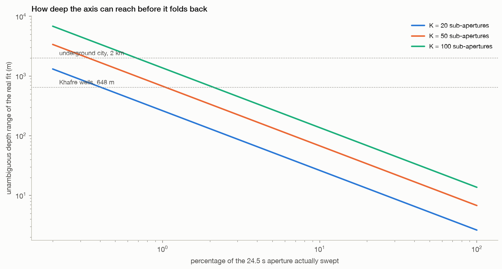
A few metres. During the 24.5 s aperture the platform moves 168 km, so a bank that uses the whole aperture spaces its steering wavenumbers very widely: at K = 50 the depth axis folds back at 6.8 m and repeats exactly at 13.6 m.

  • Depths of hundreds of metres are only reachable by sweeping about one percent of the aperture, or by enlarging the declared sound wavelength, which no measurement constrains.
  • The same calculation applies to the public derivative protocol: its shipped example assumes a one-kilometre aperture span, where the real span for that bank design is 5,006 m, so its unambiguous depth is 79 m rather than 393 m, and its shipped depth grid runs past that limit.
folds back at6.8 m
aperture for 648 m1.0%
Method, limits & data

Method. Real ICEYE X33 state vectors, Khafre RPC position and WGS84 target, aperture-centre reference. Baselines are the along-track platform offsets projected perpendicular to the line of sight, exactly as the published steering formula requires. Nyquist depth is pi divided by the median spacing of the resulting steering wavenumbers.

Leaves open. This is a statement about the ambiguity period of the steering basis under the published geometry, computed from real state vectors. It does not by itself show what a given published figure did, because the bank parameters used there were never disclosed. The comparison with the derivative protocol uses the placeholder geometry in its shipped example configuration, which its documentation asks the user to replace with real values; the point is what happens when they are replaced.

Code ↗ · Results JSON ↓

The depth axis is periodic by construction. Left: the median fit score of 200 real Khafre positions, scored by
15 · The modal branch

The modal gate picks which pixels get a depth, not which depth is right

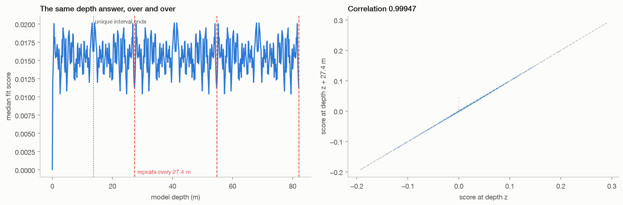
No, and it cannot. The depth stage fits each measured vector sequence to cos(Kz z) and sin(Kz z).

  • The steering wavenumbers sit on a near-regular ladder of 0.22970 radians per metre, so the two model columns at any depth z and at z + 27.4 m span the same plane, and a least-squares fit cannot tell them apart.
  • Run on real measured vectors the protocol's own focus stage scores one repeat apart at a correlation of 0.99947, which leaves only 13.7 m of depth ever distinguishable, and its own section 11.4 says so.
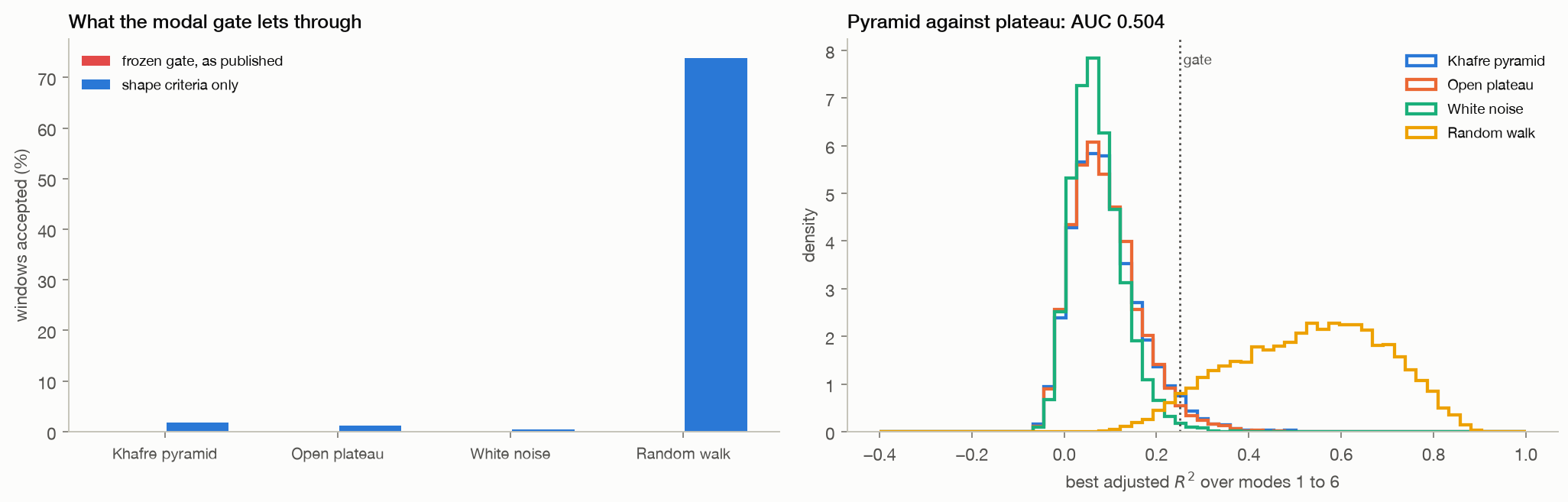
  • The modal branch runs before that stage and only decides which windows are admitted, so it changes the population and leaves the axis untouched: windows that pass the gate repeat at 0.99946.
  • The gate is not a structure detector either, since at its frozen settings it admits 0 per cent here, asking for a minor axis 25 times larger than this acquisition's displacements, and with that size threshold removed it admits 1.9 per cent on the pyramid against 1.2 per cent on open plateau, separating them at AUC 0.504 where 0.5 is a coin toss, while a random walk containing nothing at all passes 74 per cent of the time.
  • Its harmonic index counts cycles across sub-aperture position rather than vibrations in time, as the protocol's own symbol table states, and a real mechanical resonance fails separately: a chamber 30 m down rings near 18 Hz while a dwell that decorrelates in about a second carries only 0.08 to 0.51 Hz.
repeats every27.4 m
correlation there0.99947
pyramid vs plateauAUC 0.504
Method, limits & data

Method. Package v1.7 was used unmodified, with the sha256 of its modal and focus stages checked before import. Real sub-pixel registration vectors were measured on the Giza acquisition with the protocol's frozen bank design of 50 pairs, half-band masks and 88 Hz separation, at 600 positions on Khafre and the same number on open plateau. Those vectors were passed to its own modal fit at window 25 over modes 1 to 6, and to its own depth focus across three repeat lengths. Two gates are reported: the frozen Branch B rule of adjusted R-squared at least 0.25, axis ratio at least 0.1 and minor axis at least 0.005 pixels, and the same rule with the absolute size threshold removed.

Leaves open. The exact-repetition argument holds for an evenly spaced ladder of steering wavenumbers. This geometry is even to 0.0 per cent, so the repeat is very close but not perfect, which is why the correlation is quoted rather than an identity. The gate rates come from our registration vectors, not theirs, because their own registration returns whole pixels and would yield nothing to gate at all; using ours is the more favourable choice. The acquisition is an ICEYE dwell, while their frozen values describe a Capella scene, so the absolute size threshold may suit their data better than ours, and the shape-only comparison is included for that reason. The resonance figures use one representative shear speed and the simplest quarter-wave model, so they bound the band rather than predict a spectrum.

Code ↗ · Results JSON ↓

Brightness does not buy record length. Pixels of the real Khafre crop graded by amplitude, from the darkest ha
10 · Bright targets

The brightest scatterers in the scene decorrelate as fast as the desert

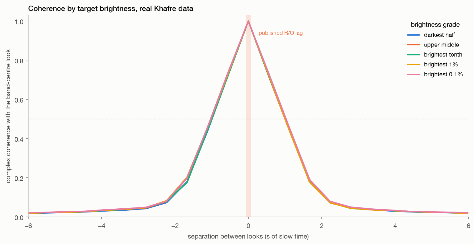
Not in this acquisition. Graded from the darkest half to the brightest thousandth of pixels, coherence with the band-centre look behaves the same way in every grade.

  • The best grade, brightest 0.1%, still retains only 0.51 at one second of separation and 0.05 at three.
  • The objection that R9's patch average is dominated by clutter, and that bright targets would do better, is not supported.
brightest 0.1%1.03 s
darkest half1.01 s
Method, limits & data

Method. 41 sub-apertures of 8% bandwidth from one real Khafre crop. Pixels graded by full-resolution amplitude percentile; up to 400 sampled per grade; complex coherence against the band-centre look accumulated over a 17 by 17 pixel window around each.

Leaves open. Giza has no deployed corner reflectors. A purpose-built trihedral, or a large stable metal structure, would almost certainly hold coherence far longer than anything in this scene, and this result does not speak to that case. Coherence is estimated in a 17 by 17 pixel window, so a genuinely isolated single-pixel target is partly averaged with its surroundings.

Code ↗ · Results JSON ↓

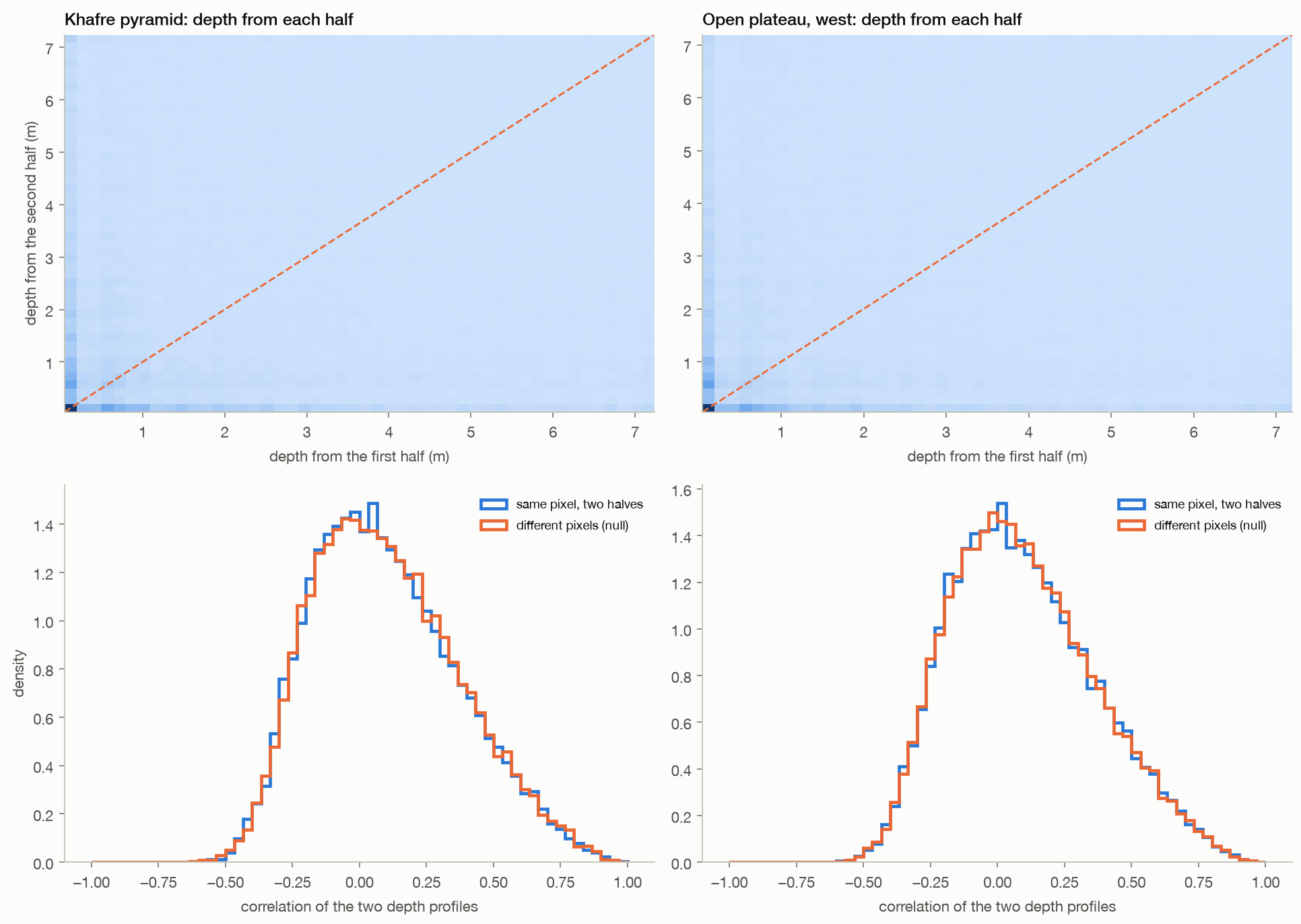
The two halves of one dwell disagree. The aperture is cut into two disjoint stretches of slow time, each given
03 · Split dwell

The first and second halves of one acquisition place the same ground at different depths

No. Splitting the Khafre dwell into two disjoint halves and giving each an identical sweep, the two halves agree on the depth of a pixel for 4.3% of pixels, against 1.3% expected by chance, and the median correlation between their depth profiles is 0.067 against 0.074 for unrelated pixels.

  • Open desert behaves the same way.
same pixel0.067
unrelated0.074
Method, limits & data

Method. One ICEYE dwell, one patch, two sub-aperture banks with identical width and swept bandwidth placed on disjoint halves of the processed Doppler support. Depth profiles are interpolated onto the shorter of the two unambiguous axes before comparison. The null is the same comparison after randomly pairing pixels.

Leaves open. Each half uses half the look angles, so each is noisier than the full sweep; some disagreement is expected from noise alone. The test shows that the depth assignments are not reproducible across look angle, not that a better estimator could not be built.

Code ↗ · Results JSON ↓

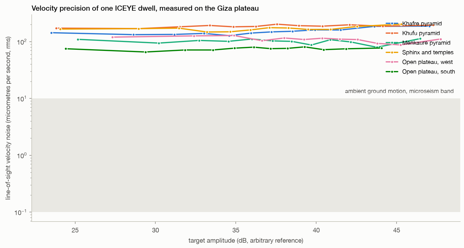
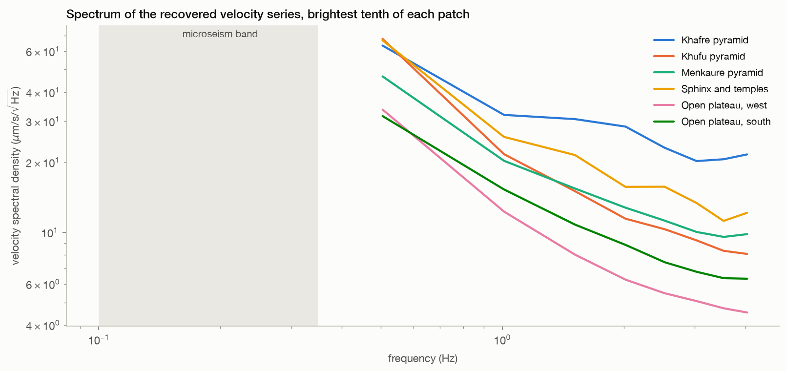
What the instrument can see. Every sub-aperture is registered against a common reference, giving each pixel an
04 · The instrument

What one dwell really measures: a velocity series, and its noise floor

A line-of-sight velocity series for every pixel, sampled at about 2.2 Hz across 22 seconds.

  • On the brightest targets in the Giza image the measured noise floor is 77 micrometres per second, and it is the same on the monuments as on open desert.
  • These looks are all kept inside the coherent window R9 measures, so the number is a measurement precision and not a decorrelation artefact.
  • The price is the span: the whole series lasts about two seconds, so the lowest frequency it can resolve is around half a hertz, above the microseism band that any passive subsurface inference would have to use.
  • Ambient ground motion in the microseism band is of order 0.1 to 10 micrometres per second, so this acquisition sits well above the motion that any passive subsurface inference would have to rest on.
  • The recovered spectra are flat and the monuments do not differ from open desert.
velocity floor77 µm/s
Method, limits & data

Method. Common-reference sub-aperture tracking: 16 sub-apertures of 8 percent bandwidth registered against the band-centre sub-aperture, all pairs kept inside the coherent window measured in R9, azimuth shift converted to velocity by v = dx V / R with the real slant range and platform speed. Spectra use a Hann window and are averaged over the brightest tenth of each patch.

Leaves open. The scene-wide median series is removed, so any motion common to the whole patch is removed with it; this bounds differential motion, not absolute platform-referenced motion. Sweeping the whole aperture instead, as an earlier version of this experiment did, produces looks that share no coherence at all and a floor that measures the search window rather than any precision; R9 gives the coherent span this bank is confined to. The floor mixes true measurement noise with real clutter decorrelation, so it is an upper bound on achievable precision rather than a fundamental limit. Corner reflectors or other strong coherent targets would do better than natural desert scattering.

Code ↗ · Results JSON ↓

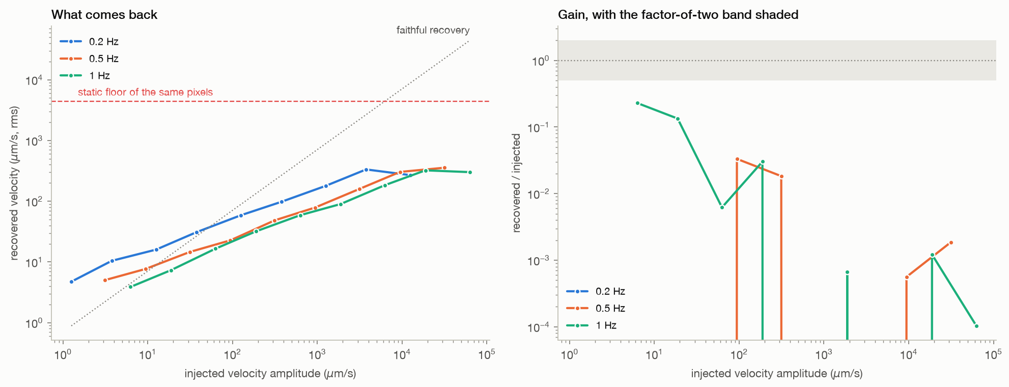
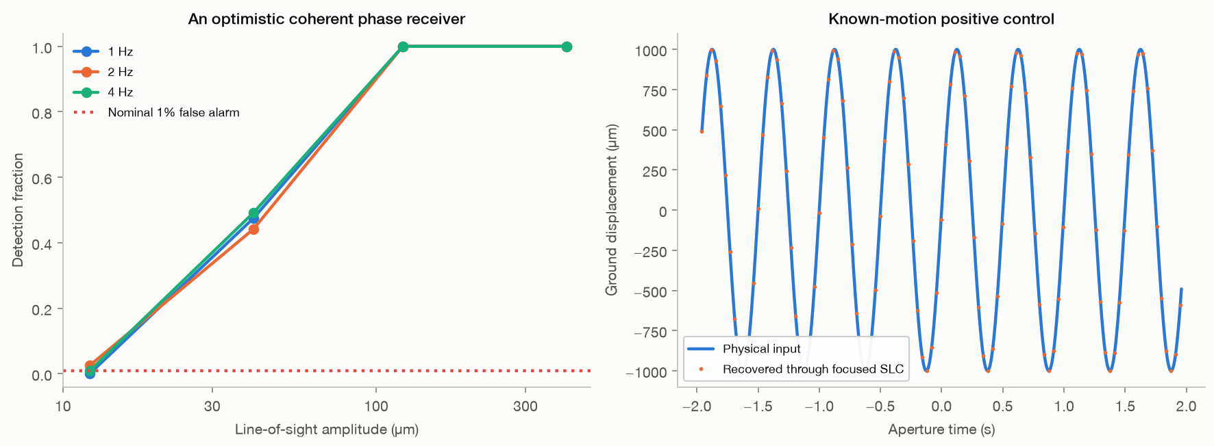
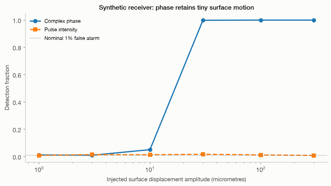
A positive control on real radar. A known line-of-sight displacement history is imposed on the Khafre crop by
07 · Positive control

Known motion put into the real image comes back, above a measurable threshold

It works, and the threshold is not reached within the tested range.

  • Below that the recovery collapses into the static floor of the same pixels, 4,397 micrometres per second.
  • Ambient ground motion in the microseism band is 0.1 to 10 micrometres per second, so the motion a passive subsurface inference would have to use sits below what this acquisition can see, on its most favourable targets.
static floor4,397 µm/s
Method, limits & data

Method. One real Khafre crop, azimuth spectrum modulated by exp(-4 pi j d(t) / lambda) with t recovered from the product Doppler rate, for nine displacement amplitudes at three frequencies. Recovery is the projection of the change in the mean velocity series onto the injected waveform, using the same fifty common-reference sub-apertures as R4.

Leaves open. The injected motion is common to the whole crop and the control therefore runs with common-mode removal disabled, which is the most favourable configuration. Real ground motion is neither spatially uniform nor single-frequency. The threshold applies to the brightest nine hundred pixels of this scene; dimmer ground is worse, and a corner reflector would be better.

Code ↗ · Results JSON ↓

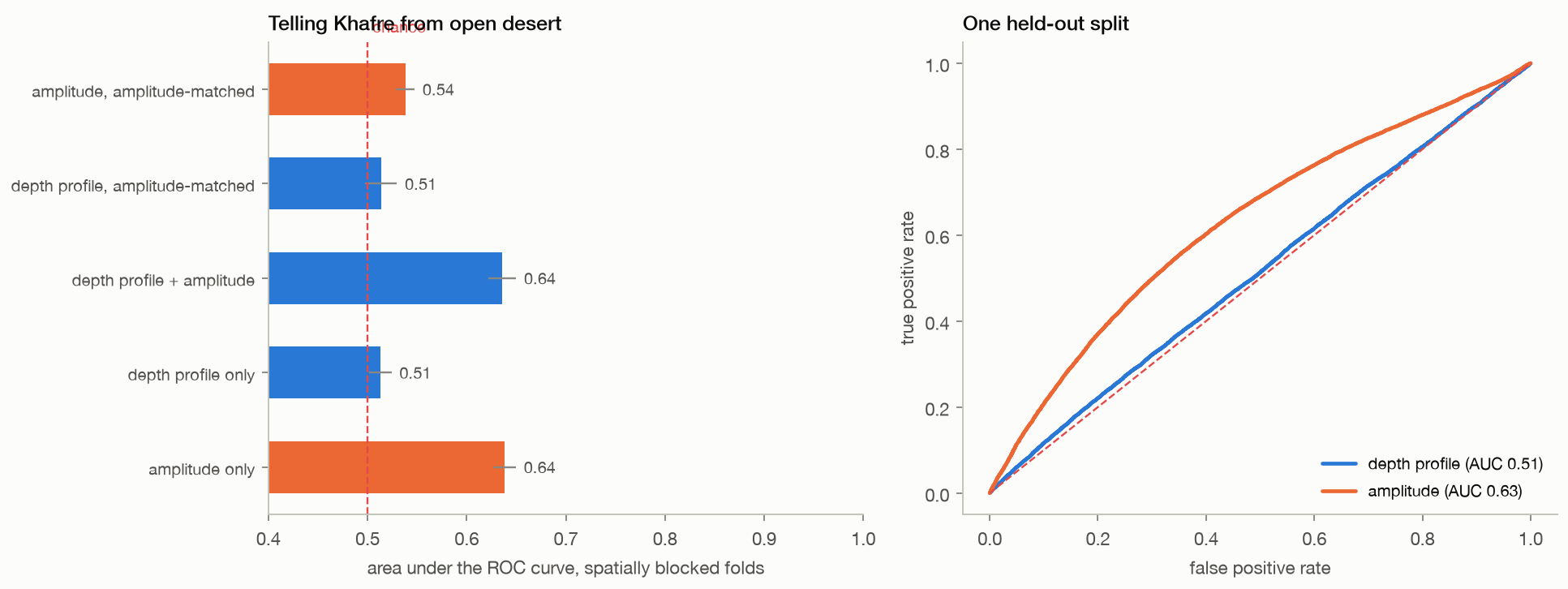
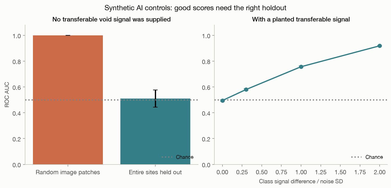
The depth axis adds nothing a brightness map does not already have. A logistic classifier is trained to separa
05 · Learned null

A classifier finds no information in the depth profiles beyond surface brightness

No. Separating Khafre pixels from open-desert pixels is an easy task and surface brightness alone reaches an area under the curve of 0.64.

  • The depth profiles reach 0.51, and once the comparison is restricted to pixels of matched brightness they fall to 0.51, which is chance.
  • Training on labelled voids would face the same problem with far fewer labels: Giza offers on the order of ten surveyed chambers, all of them under monuments, so a model would learn where the monuments are.
depth profiles0.51
brightness0.64
chance0.50
Method, limits & data

Method. Logistic regression on 32-bin normalised depth profiles and on log amplitude, scored by area under the ROC curve with five folds blocked into contiguous azimuth strips. The matched control keeps only pixels between the fortieth and sixtieth percentile of brightness.

Leaves open. A linear model on binned profiles; a larger network could fit more, but with spatially blocked folds and a matched-brightness control there is little left for it to fit. The test shows an absence of separable information in these features, not a proof that no representation could ever separate them.

Code ↗ · Results JSON ↓

12 · Independent code

The derivative protocol's own code, run unmodified on the real acquisition

No. Version 1.7 of the public derivative protocol was installed unchanged, its own tests passed, and it was given a real Khafre crop with an honest configuration.

  • It runs.
  • Its registration returns only the integer peak of the cross-correlation, so the displacement vectors it feeds to the depth fit are whole numbers of pixels, with 1 distinct values across the whole target track.
  • Real inter-look displacements in this data are thousandths of a pixel, so that estimator quantises the entire measurement to zero.
  • Its geometry is also misconfigured by default: the shipped example assumes a 1 km aperture span where the real span for that bank is 9,868 m, which moves its recurrence depth from 494 m to 50 m, below the 100 m grid it searches.
distinct vector values1
its depth grid100 m
its real limit50 m
Method, limits & data

Method. v1.7 installed from its published package and run through its own command line on a 1024 by 512 complex crop of the real Giza product, twice: once with the aperture span its example assumes and once with the span derived from the product state vectors.

Leaves open. Our configuration is not theirs. Target track, nuisance arcs, patch size and depth grid were chosen by us from the shipped example, because the settings behind the published images were never released. This shows what their code does on real data under a reasonable configuration, not that any particular published figure came from it.

Code ↗ · Results JSON ↓

Simulation · 8 tests

What the method computes, in scenes whose contents are known

Synthetic scenes establish the mechanism: a motionless pyramid, empty desert, two rocks, ground that really moves.

01 · Static scene

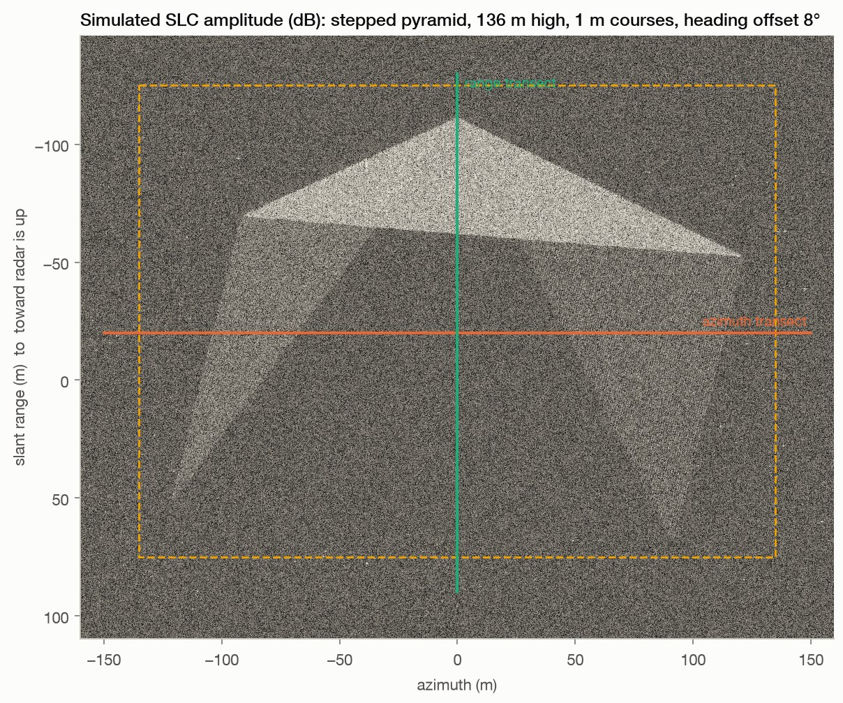
A stationary pyramid produces depth-like patterns

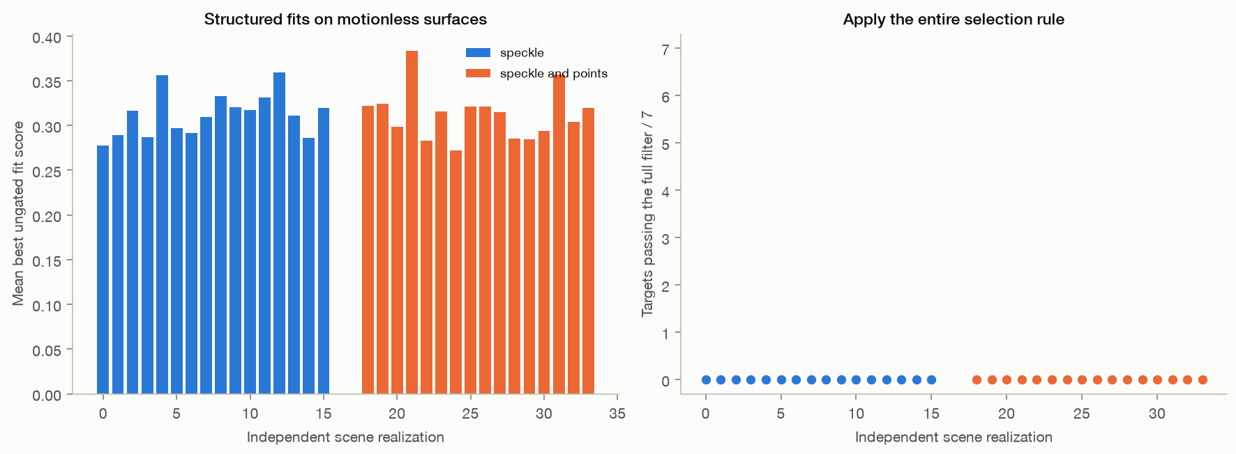
The reconstructed pipeline produces layered patterns although the simulated scene has no motion or subsurface.

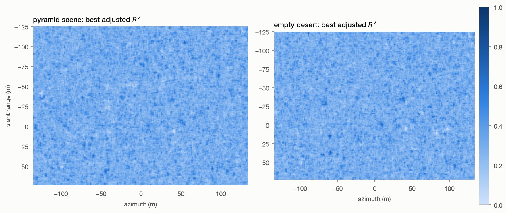
  • Mean best window-fit scores are 0.306 inside the ground footprint and 0.308 outside it.
Method, limits & data

Method. Scene: 348,713 point scatterers (course edges with aspect-dependent 'flash', diffuse face scatter, rocks) plus speckle clutter, synthesised into a 1280 × 1024 SLC. Pipeline: K = 50 reference/offset sub-aperture pairs (half-band, 88 Hz offset snapped to 4 FFT bins), 32 × 32 complex cross-correlation to 1/1000 px, global common-mode removal, λₛ = 0.48 m. Grid: 54,000 pixels at 1 m, run time 4.4 min.

Leaves open. One stylized scene and one random seed. The footprint is a ground-plane mask, not a scatterer attribution map: layover mixes locations. A high fit score is not a probability of a buried structure.

Code ↗ · Results JSON ↓

02 · Null control

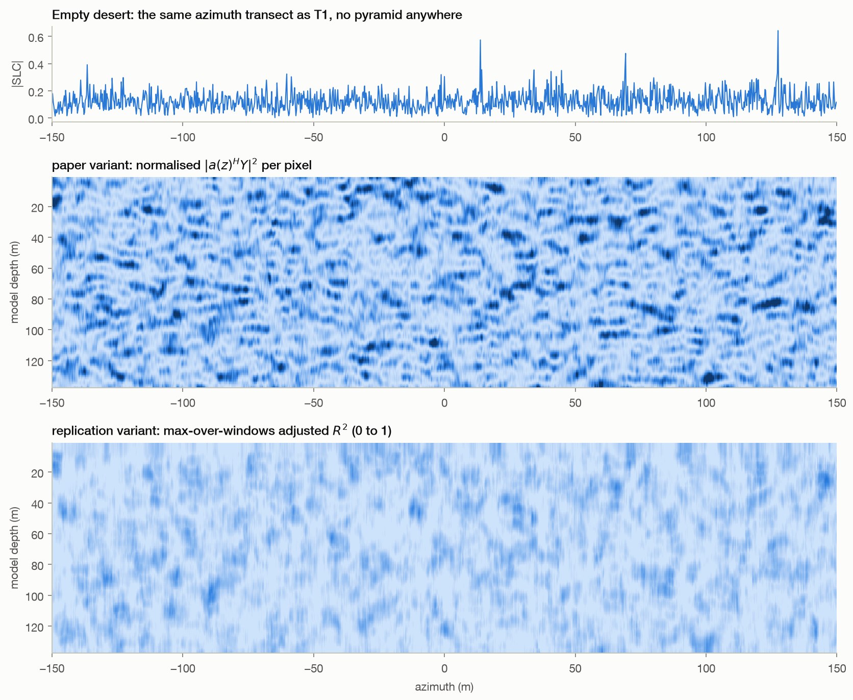
Empty desert produces a similar score distribution

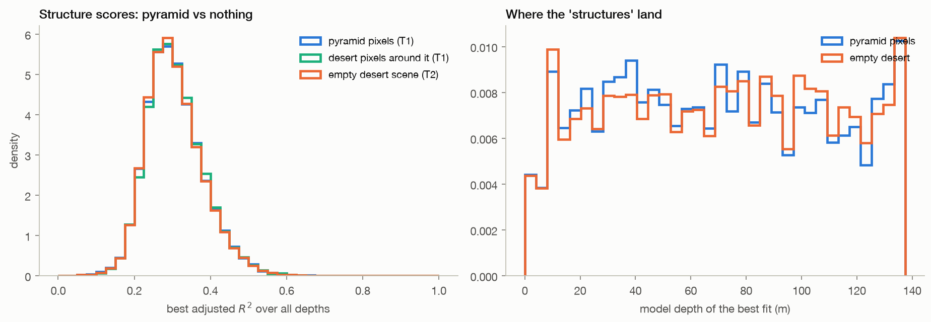
The mean best score is 0.306 on the pyramid footprint and 0.306 in the desert-only scene.

  • Their empirical distribution distance is 0.0096.
  • The absence of buried objects does not prevent structured output.
Method, limits & data

Method. Identical pipeline and grid as T1 on a scene containing only clutter and sparse rocks; scores compared pixel by pixel with T1's pyramid footprint.

Leaves open. One realization per scene; the 32-pixel patches overlap on a 4-pixel grid, so the samples are dependent. The saved conventional KS p-value is descriptive only here. Similar distributions do not establish statistical equivalence or validate a detector.

Code ↗ · Results JSON ↓

03 · Mechanism

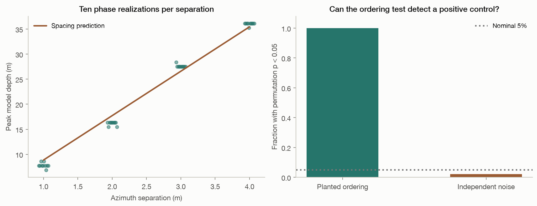
Surface spacing predicts the apparent depth

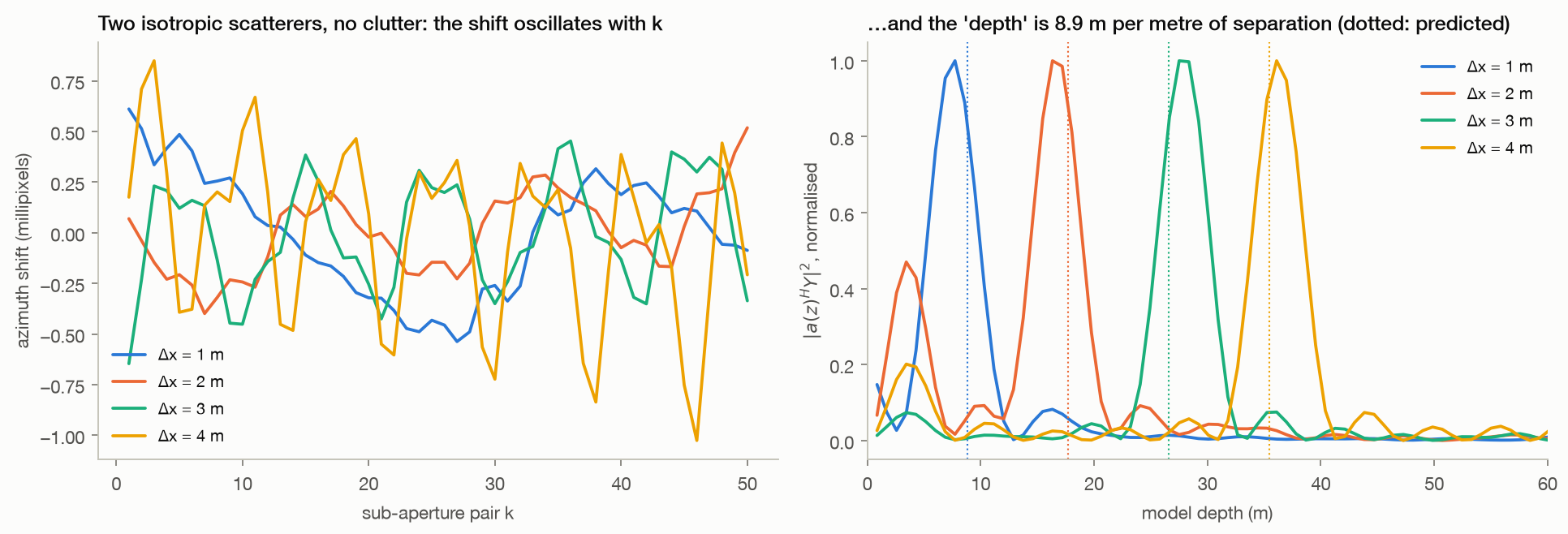
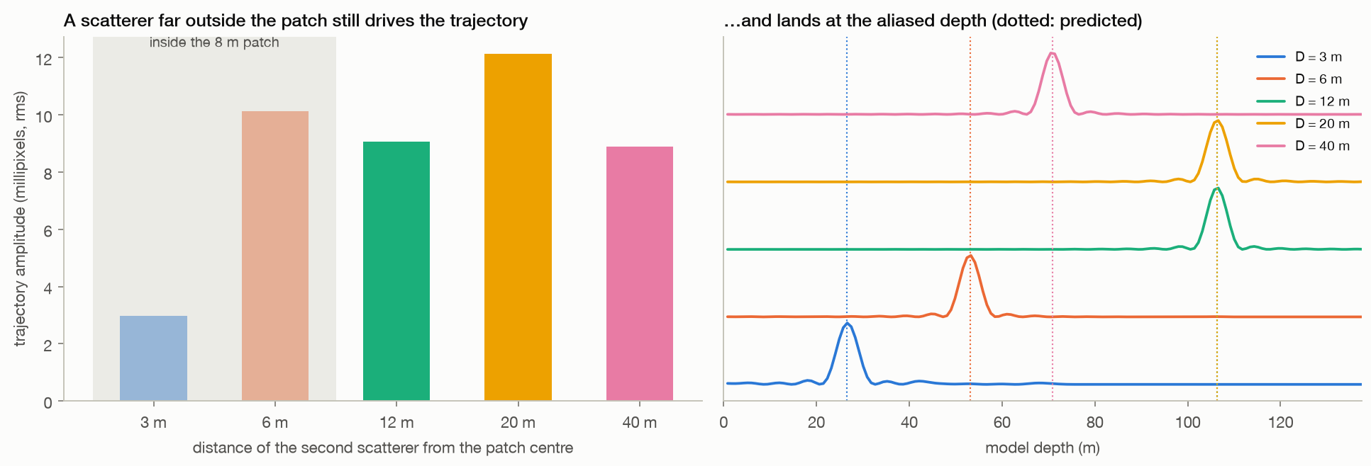
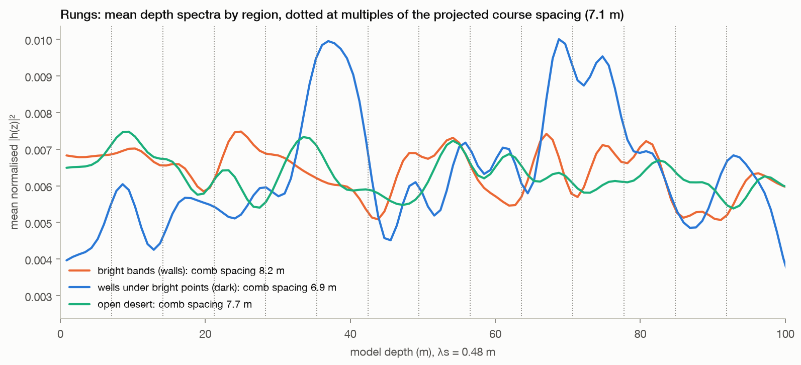
In the two-scatterer examples, peak depth tracks azimuth separation at approximately 8.86 model-metres per metre.

  • Farther scatterers can contribute outside the patch, and the sampled depth axis folds high spatial frequencies back by aliasing.
Method, limits & data

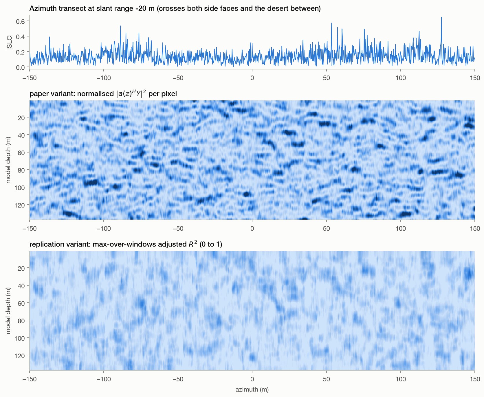
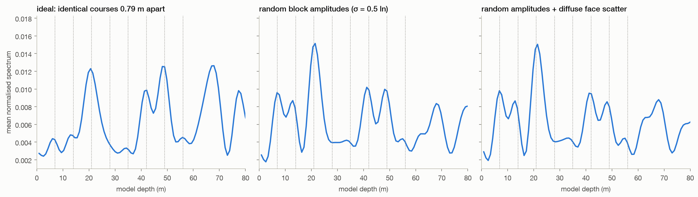
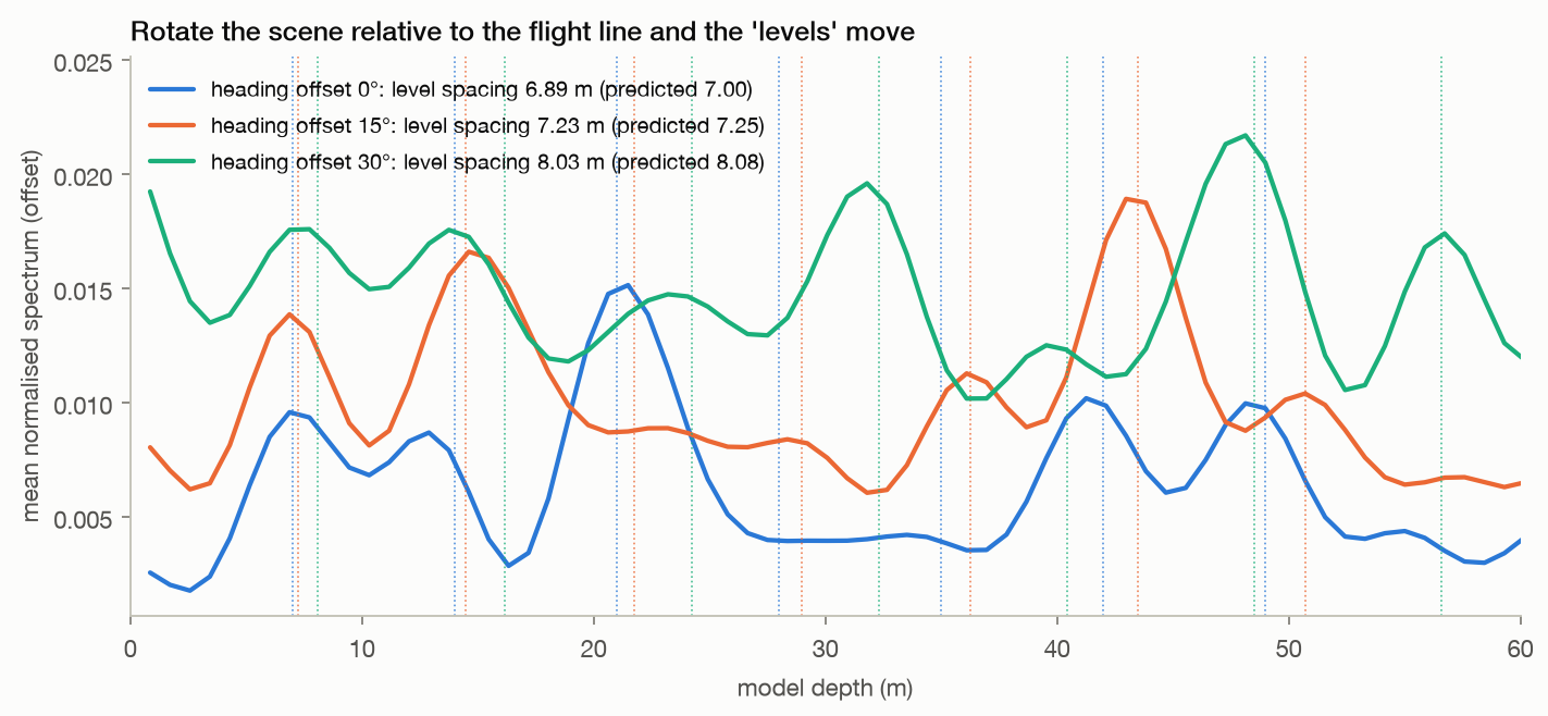
Method. Clutter-free two-scatterer scenes at 1, 2, 3, 4 m separation and at 3 to 40 m; a 60-line periodic wall in three degrees of realism; the realistic wall at three headings with a harmonic-comb fit of the level spacing. Same bank and patch as T1; transect spectra averaged over 160 pixels.

Leaves open. Ideal point scatterers and a prescribed spectral model. The wall's comb fit depends on reflectivity: the ideal-wall fitted spacing differs from the prediction, while the randomized variants are closer. These examples identify a mechanism in this reconstruction, not the cause of a particular published feature.

Code ↗ · Results JSON ↓

04 · Processing choices

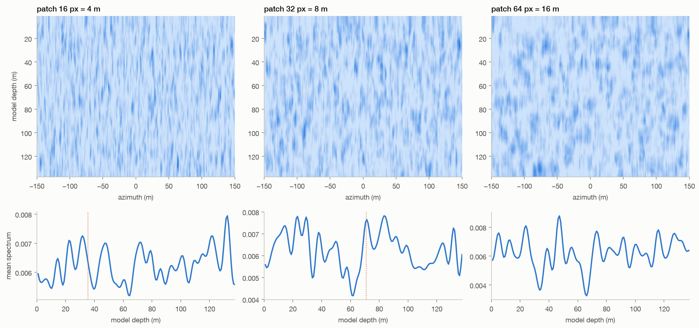
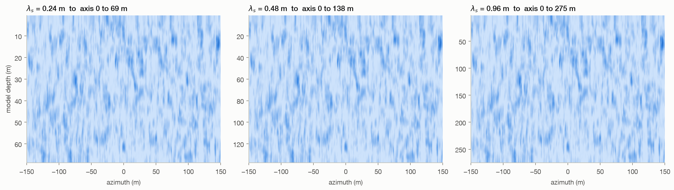
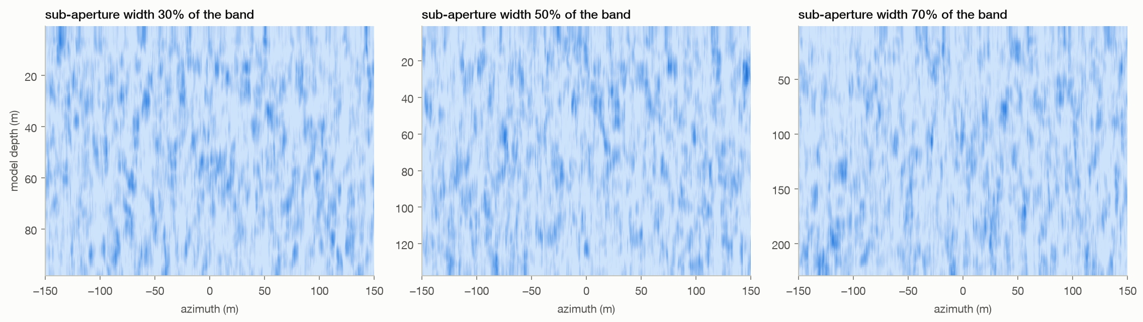
Processing choices set the axis and change the patterns

Patch size changes spatial smoothness.

  • The declared wavelength scales the model-depth axis, and the sub-aperture width changes its sampling and the resulting pattern.
  • The wavelength panel illustrates an exact algebraic rescaling; a separate end-to-end test verifies that relation.
Method, limits & data

Method. Desert and pyramid transects with patch widths 16, 32, and 64 pixels and sub-aperture fractions 30%, 50%, and 70%. The wavelength panel relabels a single computed result at 0.24, 0.48, and 0.96 m. Band edges are snapped to FFT bins.

Leaves open. One scene per sweep, with one parameter changed at a time. Sensitivity alone does not invalidate an inverse method; the relevant question is whether calibrated, independently validated targets remain correctly localized. No such validation is supplied by this experiment.

Code ↗ · Results JSON ↓

05 · Injected motion

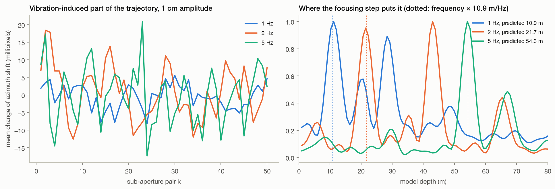
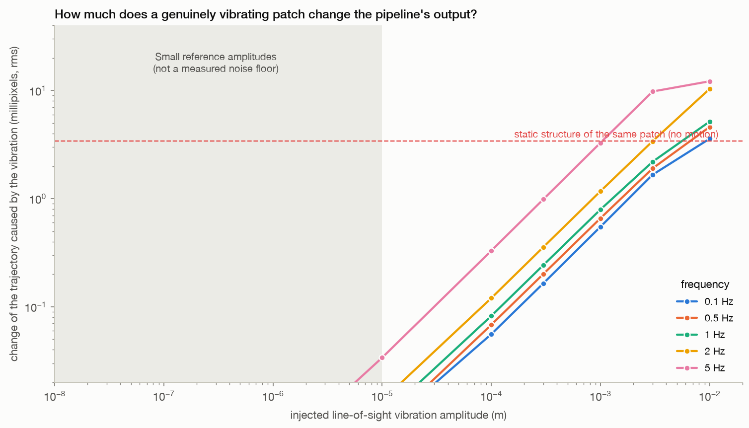
Motion changes the output; frequency becomes model depth

At 1 cm imposed amplitude, the response reaches 3.58 times the static trajectory rms.

  • The focusing step places vibration near 10.87 model-metres per hertz; the 2 Hz case peaks at a second harmonic.
  • This is a response measurement, not a calibrated detection limit.
Method, limits & data

Method. Static desert SLC plus a synthesised vibrating patch (linear superposition), 5 frequencies × 7 amplitudes from 1 µm to 1 cm; response measured as the change of the sampled patch trajectories relative to the same patch at rest, compared with the rms of the static trajectories.

Leaves open. One sinusoidal patch and static background clutter. Subtracting the exactly known motion-free baseline is an advantage available in simulation. No sensor-noise distribution, false-alarm calibration, or cavity-to-surface model is included. The result does not establish a general limit on radar vibrometry.

Code ↗ · Results JSON ↓

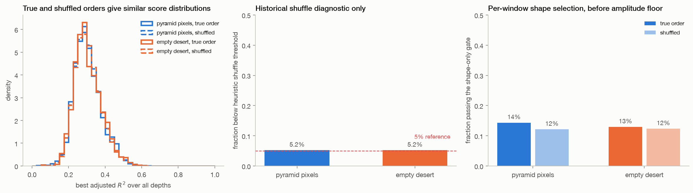
06 · Ordering & gates

The full ellipse gate rejects the sampled static pixels

The corrected per-window shape gate accepts 14.3% of pyramid and 12.9% of desert pixels.

  • After the 0.005 px minor-axis floor, the full gate accepts 0.0% and 0.0%.
  • The earlier shuffle comparison is retained as a diagnostic only.
Method, limits & data

Method. For each of 26 contiguous W25 windows, choose the best ellipse mode from 1–6, then apply adjusted R² ≥ 0.25, axis ratio ≥ 0.1 and minor axis ≥ 0.005 px. Pixel acceptance requires at least one fully accepted window. Legacy shuffle results use 60 arbitrary order permutations and are descriptive only.

Leaves open. One scene per class and 1,500 dependent pixels. Arbitrary look permutations change correlations between overlapping sub-apertures, so the shuffle statistic is not a calibrated physical null test. The new independent-scene controls replace it as the primary null comparison. Shape-only acceptance is not a false positive of the full gate; sensitivity must also be tested on physical positives.

Code ↗ · Results JSON ↓

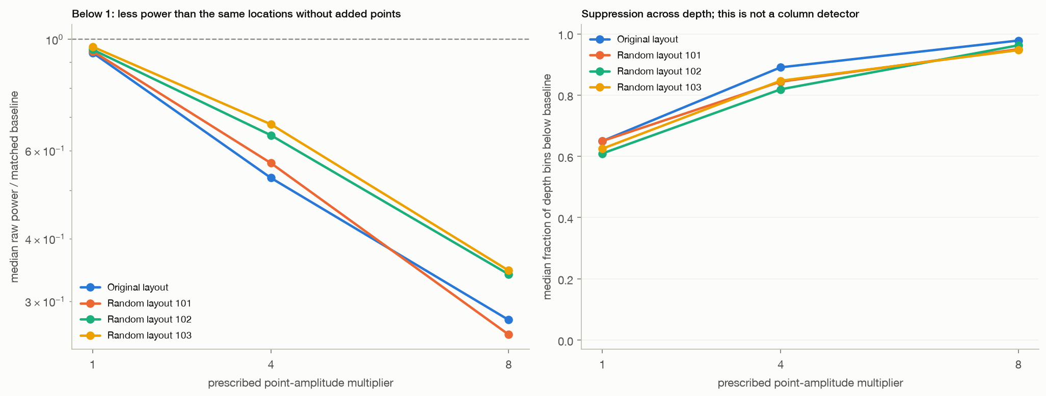
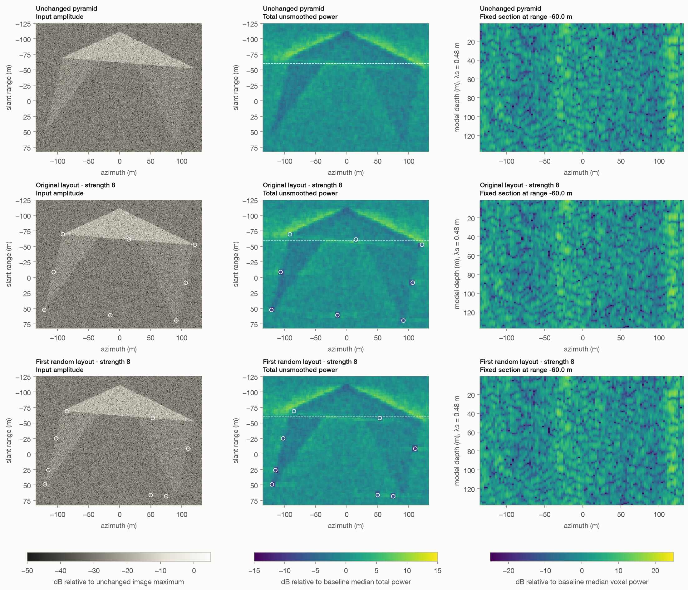
07 · Paired surface controls

Add surface targets; measure what changes before rendering

At strength 8, median unsmoothed power near the original eight points is 0.28 times the same locations in the unchanged pyramid.

  • Across the three random layouts it ranges from 0.26 to 0.35.
  • The implemented full gate accepts no sampled pixels in any of the 13 scenes.
Method, limits & data

Method. Thirteen paired scenes: unchanged pyramid; original corner/midpoint layout at multipliers 1, 4 and 8; three random perimeter layouts at those same multipliers, with seeded relative amplitudes uniform on [0.5, 1.5]. All reuse the same pyramid, clutter seed, point phases, radar geometry, 50 sub-aperture pairs, 32-pixel patches, 2.5 m target grid, common-mode rule, 0.48 m wavelength and 160 model-depth bins. Regional raw power is compared with the identical baseline pixels in fixed 8 m squares. The T6 shape and full gates are applied to every grid trajectory. No smoothing, isosurfaces, per-scene normalization or depth rescaling is used. The displayed random example is always seed 101.

Leaves open. One background realization, three random perimeter layouts and ideal point targets with prescribed amplitudes. Added points have no terrain-shadowing or object-specific scattering model. Spatial samples overlap, and strength variants reuse the same layouts. Power changes and depth-bin suppression are descriptive responses, not validated column detections. Neither the point count nor the output depth limit predicts a Khafre structure. This tests our reconstruction and T6 gate implementation, not the original data or complete Khafre workflow.

Code ↗ · Results JSON ↓

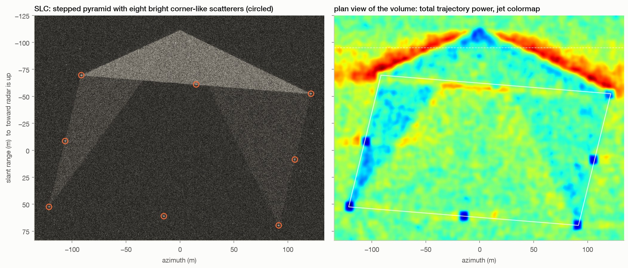
Appendix · Constructed rendering

Illustration: surface points and rendering choices

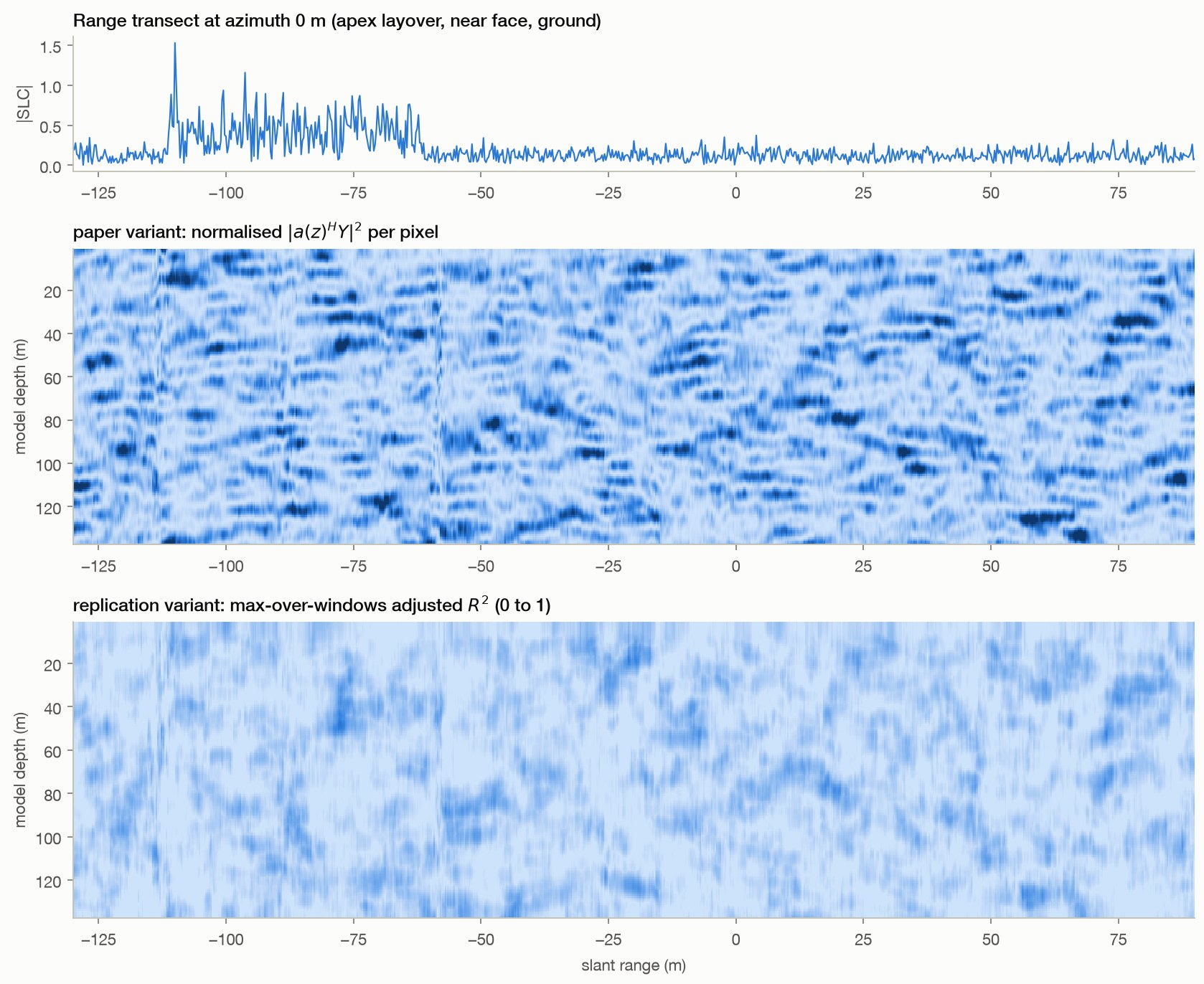
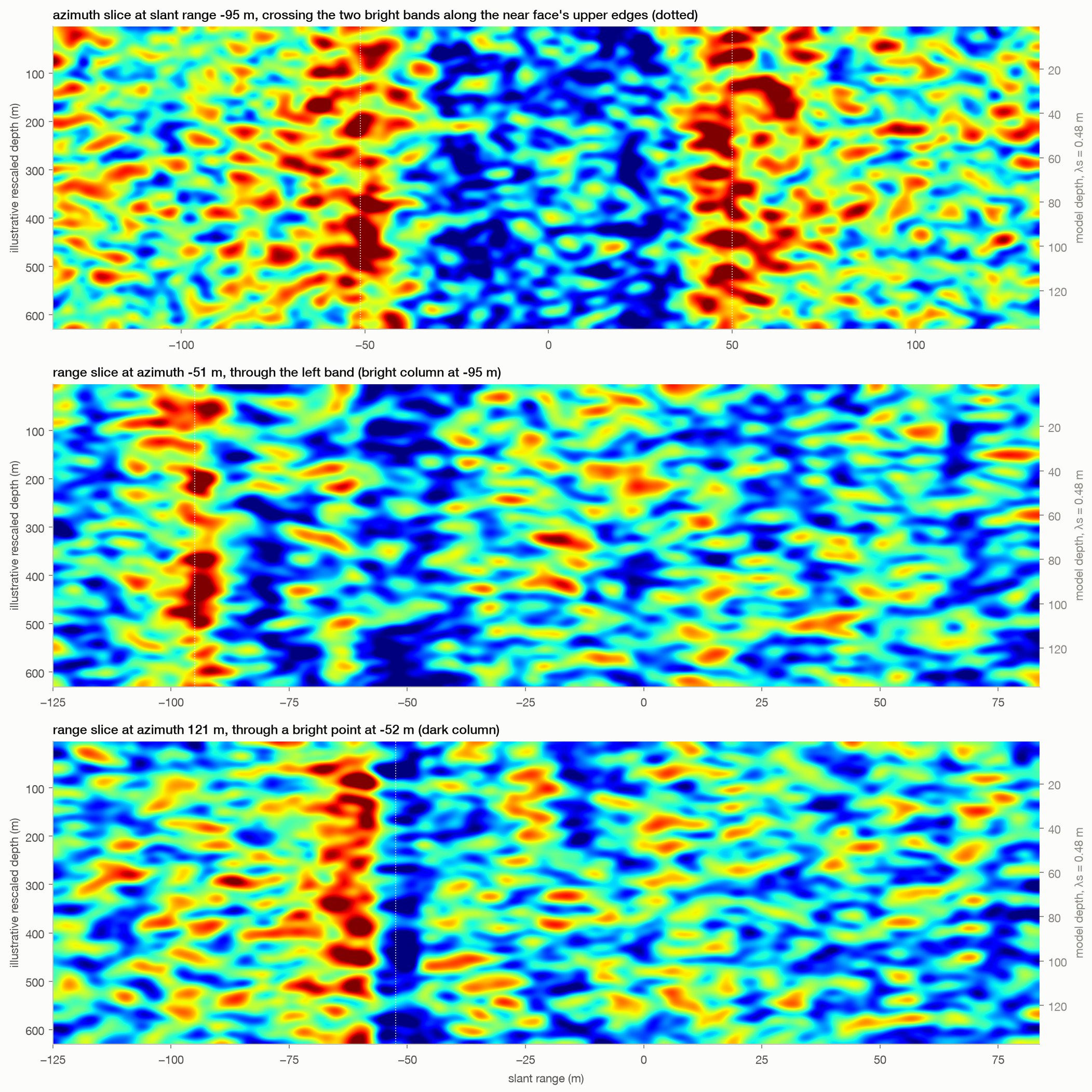
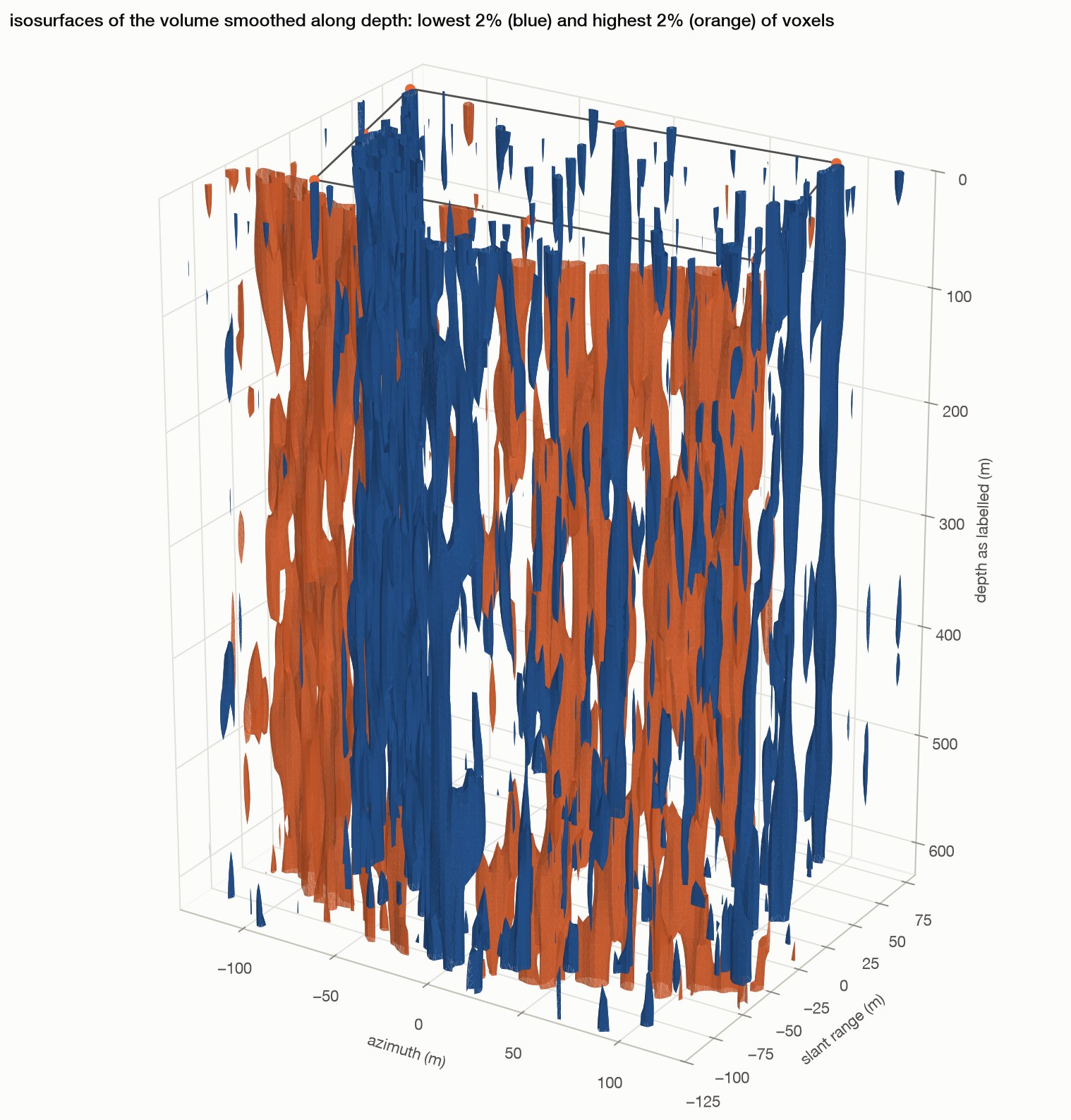
In this constructed scene, dominant point scatterers produce dark columns (0.20 times desert power), while mixed face edges produce bright bands (4.84 times desert power).

  • The displayed volume ends at 137.5 model-metres, or 630.4 m after a chosen wavelength rescaling.
Method, limits & data

Method. T1's pyramid plus eight point scatterers of amplitude 8 at the base corners and mid-edges; paper-variant volume on a 1.25 m grid (36,000 pixels); log-magnitude smoothed with a Gaussian of 1 sample in position and 1.5 in depth; jet colormap and bicubic interpolation to match the published rendering; marching-cubes isosurfaces at the 2nd and 98th percentiles of the volume smoothed along depth.

Leaves open. Eight bright points are placed by hand. The 2.2 m wavelength, smoothing and display thresholds are chosen for illustration. This example does not apply T6's acceptance gate. Neither the point count nor the roughly 630 m display floor is an independent prediction. Visual resemblance does not establish the origin of the Khafre features, validate the surface targets' realism, or reproduce the original processing. This illustration neither reproduces nor measures spiral ramps.

Code ↗ · Results JSON ↓

Supporting · 3 results

Where the method is given every advantage

A coupled physical benchmark, the measurement chain it rests on, and the stress tests behind the simulated examples.

Steelman · coupled benchmark

Given a favourable physical model, depth is recoverable

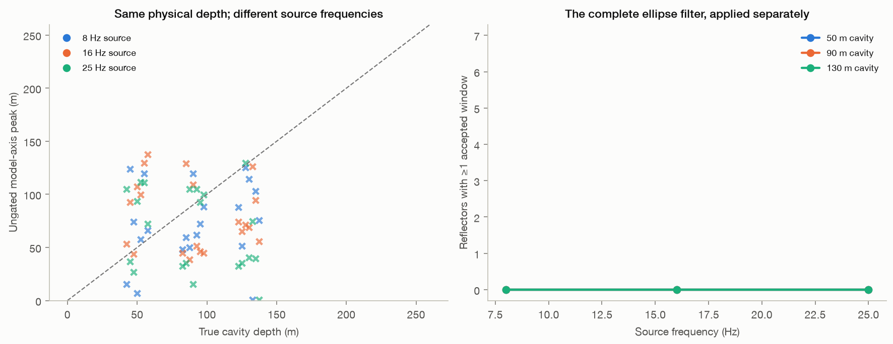
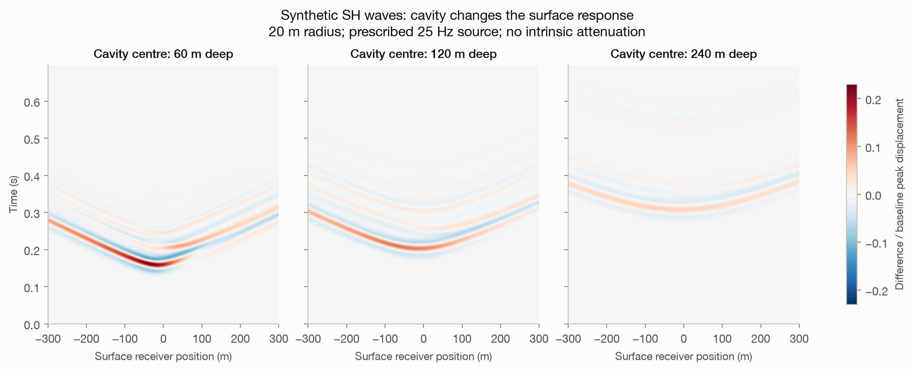
A buried cavity drives a wave-equation forward model, the surface motion modulates a radar acquisition, and a physical-template inverse recovers the depth.

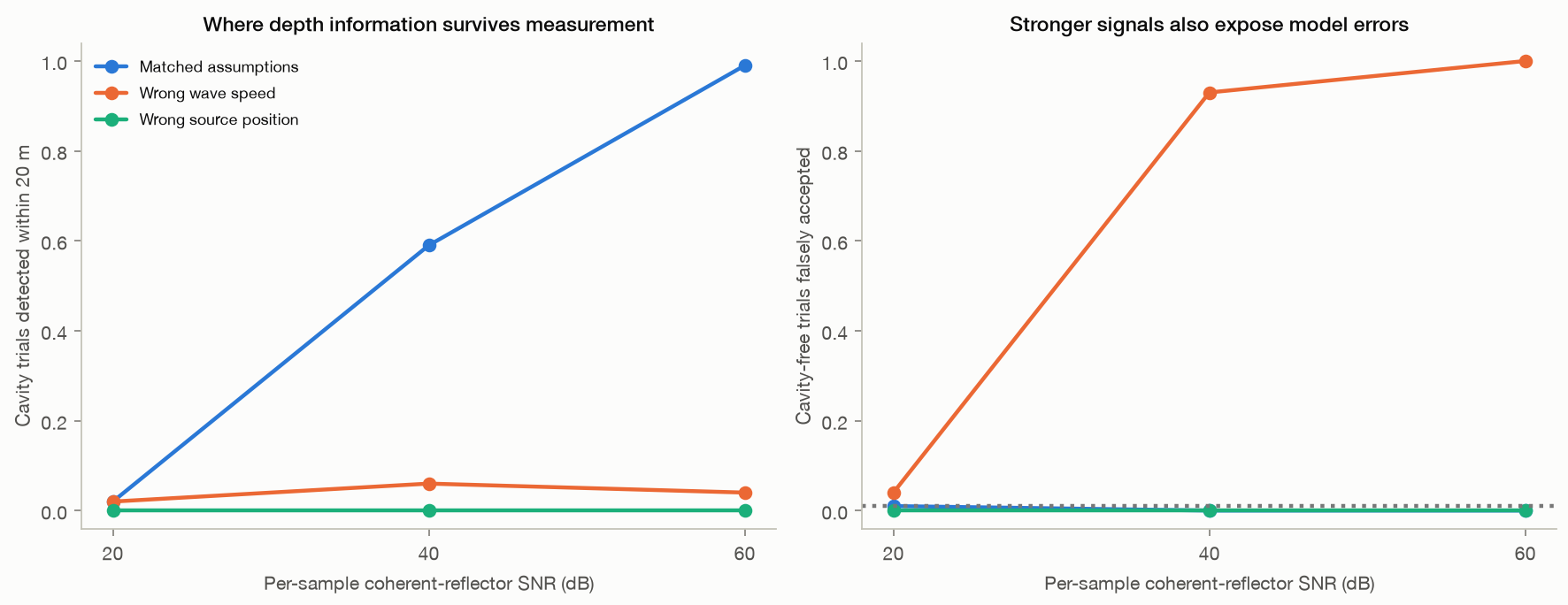
  • At 60 dB channel signal-to-noise, 99% of trials locate the cavity within 20 m, with a 0% false-alarm rate.
  • At 20 dB that falls to 1%.
  • The forward model never uses the Doppler-to-depth steering formula, so this is an independent check that depth information can survive in principle, not a vindication of the published method.
  • It assumes a known active source, uniform rock, a horizontal cylindrical void and favourable readout. None of those hold at Giza.
high SNR99%
low SNR1%
Figures & code

Code ↗ · Results JSON ↓

Steelman · measurement chain

The phase channel and its units work in a controlled acquisition

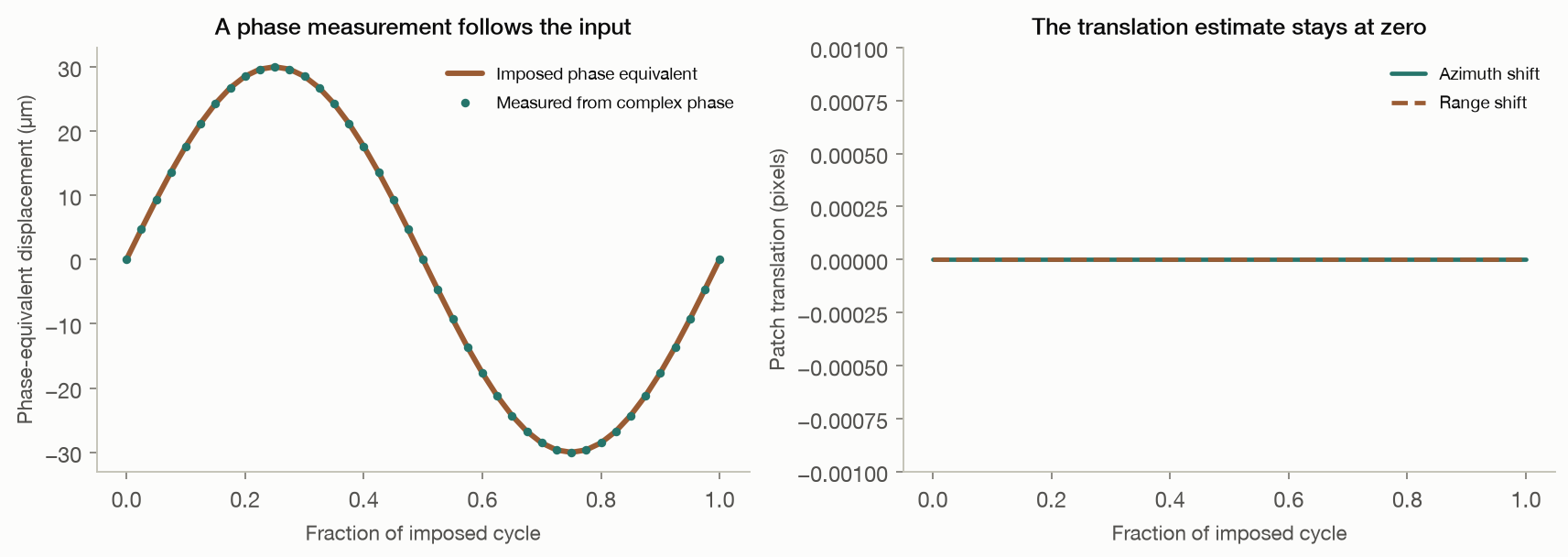
A known displacement passes through focusing and is recovered from the complex image.

  • Positive controls confirm phase, sign and units survive an idealised focusing operation.
  • Artificial detection datasets isolate the confounding a learned detector would face.
  • These are favourable resolved targets and perfect platform compensation, not distributed pyramid scattering.
Figures & code

Code ↗ · Results JSON ↓

Controls · stress tests

The simulated examples survive repetition and reseeding

Across 40 two-scatterer runs the median peak sits 0.92 m from the spacing prediction, at most 2.25 m.

  • The permutation test flags 100% of planted ordered trajectories and 2.1% of pure noise, at a nominal 5 per cent level.
  • End-to-end reruns at three declared wavelengths reproduce the predicted rescaling.
median error0.92 m
worst2.25 m
Figures & code

Code ↗ · Results JSON ↓

Falsification

What would change this conclusion

Stated in advance and in testable form. Any one of these, demonstrated, would reopen the question.

A positive control succeedingLocate a surveyed void at its known position with the processing settings frozen beforehand, and score the result against chance. R13 does this at cemetery scale and finds nothing; a single named chamber needs metre-level registration, which is the next task on the roadmap.
Depths that reproduce across look angleSplit one acquisition into two disjoint halves, give each an identical sweep, and show that the same ground is placed at the same depth by both. R3 measures a correlation of 0.067 between halves against 0.074 for unrelated pixels.
Depths that survive their own free parametersShow a feature whose depth does not move when the declared sound wavelength or the sub-aperture width changes. At present the depth axis scales linearly with a constant no measurement constrains.
Coherence on a target class we have not measuredA deployed corner reflector, or any target holding complex coherence beyond a few seconds of look separation, would lengthen the usable record and weaken R9 and R11. Nothing in either scene does.
Agreement between two acquisitions of the same groundTwo dwells of the same plateau on different dates should place the same structure at the same depth. We hold one acquisition per site and cannot run this; it is the cleanest test we are missing.
Scope

What this does and does not claim

Worth reading before drawing a conclusion from anything above.

Measuring vibration from radar is real

Estimating micro-motion from SAR sub-apertures is established and works: on ships, bridges and other strong, stable structures vibrating fast enough that very short lags suffice. Independent work in 2026 recovered 1 to 4 Hz motion on controlled reflectors. Nothing here questions that. The subsurface claim is a different regime in every variable that matters: a distributed natural target, a frequency band a hundred times lower, and an inference about depth rather than about motion.

No published figure is reproduced here

The sub-aperture parameters, patch positions, nuisance geometry and wavelength model behind the Khafre images were never released, so no result on this page reproduces a specific published image. Everything reproduces the method as described, with settings chosen and published here. If the disagreement lies in those settings, releasing the originals would resolve it quickly.

The public derivative protocol, run unmodified

Version 1.7 of the openly published derivative protocol was installed without changes, its own tests passed, and it was given a real Khafre crop. Its registration returns only the integer peak of the cross-correlation and produced one distinct displacement value across an entire target track, where real inter-look displacements are thousandths of a pixel. Its example geometry also assumes a one-kilometre aperture span where real state vectors give about ten, moving its ambiguity limit from 494 m to 50 m, below the 100 m grid it searches. Both are fixable.

Everything is open and rebuilds from source

The two radar products are commercial acquisitions and are not redistributed, but every script, configuration, intermediate result and figure is in the repository, and this page is generated from the saved reports. Corrections to earlier versions of this work, including two of our own mistakes, are kept in the method audit. Disagreement is best expressed as a rerun.

Reproduce any number on this page

git clone https://github.com/ejhong/sar && cd sar
python3.11 -m venv .venv && .venv/bin/pip install -r requirements.txt
.venv/bin/python -m pytest tests                      # 80 tests

cd experiments && ../.venv/bin/python run_all.py      # simulation chapter, self-contained
../.venv/bin/python r13_known_voids.py                # needs the ICEYE products
cd .. && .venv/bin/python build_dashboard.py         # rebuilds this page

Product paths are in experiments/real_common.py. Nothing reads a full raster; every step works on a bounded, geolocated crop and records its origin. What is and is not established, including corrections to our own earlier results, is kept in METHOD_AUDIT.md.

Method

What was run

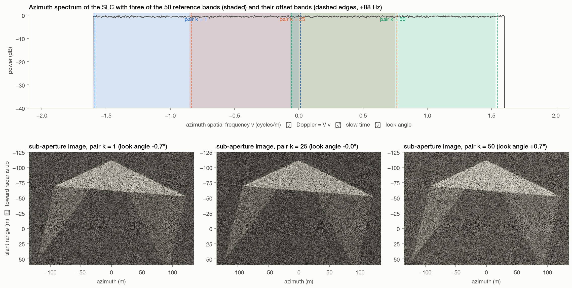
Sub-apertures. Top: the image's azimuth spectrum, whose axis is simultaneously Doppler frequency, slow time along the 3.9 s aperture and look angle across 2.8°. Three of the fifty reference/offset band pairs are drawn. Bottom: the pyramid seen through those three bands. Each is a lower-resolution image from a slightly different angle; the speckle and the bright block facets change between them. The pipeline's 'micro-motion' is the sub-pixel shift between the reference and offset versions of each 32 × 32 patch, tracked across the fifty pairs.
AcquisitionsICEYE X33 Giza 2025-08-27 · ICEYE X35 Sacsayhuamán 2025-08-22, Spotlight Dwell Fine, VV
Image113,692 × 11,562 complex samples, 0.044 m azimuth, 0.154 m slant range
Aperture24.5 s of slow time carried on the Doppler axis; the image row span is 0.713 s and is not the aperture
Sub-aperturesReference and offset passbands swept across the processed band; the published designs overlap 96–99% at lags of 14–72 ms
Registration32 × 32 complex cross-correlation, upsampled DFT to 1/1000 px, validated on this radar texture with planted shifts down to 0.005 px
Depth geometryKz = 4π B⊥ / (λs r sin θ) with B⊥ the along-track platform offset from the product's own 101 state vectors, not a scalar approximation
Depth conventionπ/ΔKz is the range a real two-component fit can use; the complex output repeats at twice that

Sources